It is easy to ignore the option value when providing liquidity (LP for liquidity provider) because this is second-order relative to the risk from the price of one’s assets changing. Consider an unrestricted range where one provides $500k in ETH and USD at an initial price of $2500. The initial position is represented by the black line, the pool position by the red, and the impermanent loss (IL) is the difference between the two.
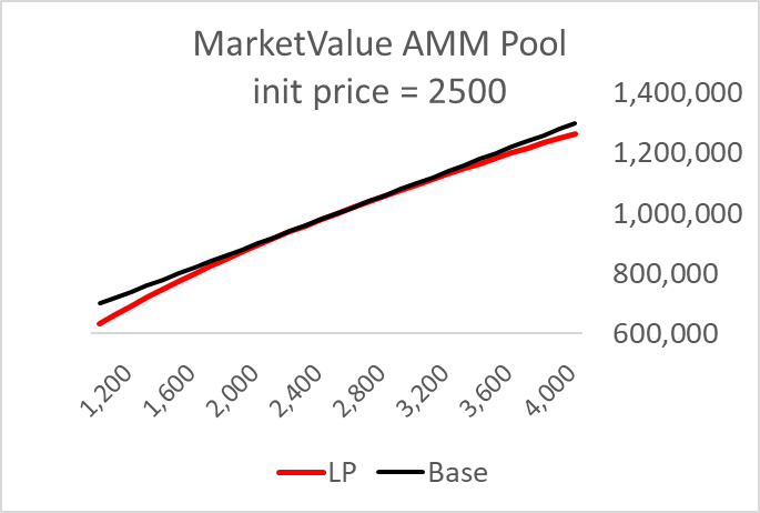
Another way to see this second-order distinction is by comparing that difference, the IL, with the pnl of the initial position. The orange line seems almost irrelevant. Almost.
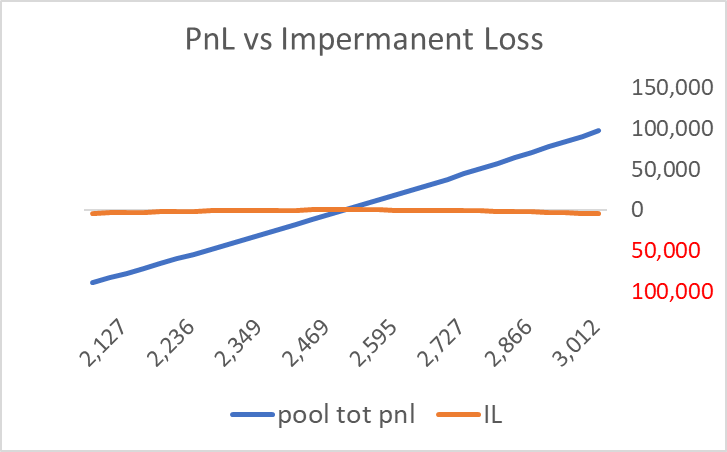
It turns out that the IL will cost you around 12.5% annually for a token with a 100% annualized volatility (ETH’s vol is about 90%). Many people are being fleeced because they only look at the fee income in these pools.
The current automated market maker (AMM) LP situation is reminiscent of convertible bonds, where the seller of the bond includes an option for the buyer. If the stock price goes up, the bondholder can exchange his bond for a share of stock. As the value of this option is positive to the buyer, this lowers the bond issuer’s yield, seemingly saving the company money via a lower interest expense. Many ignorant Treasurers reasoned, “if the price goes up a lot, my shareholders will be happy, so they won’t be mad at me for some opportunity cost via dilution. If the price goes down, the shareholders will be happy because I saved the company money by selling a worthless option. Win-win!”
For decades convertible bonds were underpriced because their option value was undervalued, driven by the ignorant reasoning above. Savvy investors like financial wizard Ed Thorpe bought these bonds, and when hedged within a hedge fund, this strategy generated consistent Sharpe ratios near 2.0 without any beta through 2004. Eventually, investment banks became good at separating the options from these convertible bonds via derivatives, which made the value of the options within these bonds more transparent. Competition via arbitrage strategies pushed convertible bond prices up to accurately reflect the value of this option, and the days of easy alpha in convertible bonds were over.
An LP offers a pair of tokens for people to buy or sell at a current price. If you provide ETH and USDC to a pool, you implicitly offer a fixed price for buy or sale at every instant. In a limit order book, it would be analogous to offering to buy or sell Tesla at $750 when the current price is $750. If you leave that offer out there for a week, clearly, you will have bought only if the price went down and sold only if the price went up. This is called ‘adverse selection,’ because your offer selects the trade that is adverse to you.
Uniswap’s AMM isn’t exactly the same because the quantities offered do not have a fixed price, but the general idea is the same. It is like selling a put and a call at a fixed price, also known as a short straddle.
A short straddle payout looks like this:
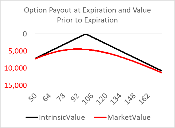
The payout for a short straddle is strictly negative, but the option is sold for a positive amount. In equilibrium, the price should be slightly above the average payoff to compensate the seller for taking on risk, as potentially the seller could lose a lot of money. In contrast, the option buyer can only lose precisely as much as he paid. This risky nature of the option seller’s position is reflected in its convexity. The seller is exposed to negative convexity (second derivative negative) while the buy gets positive convexity. Positive convexity is like a lottery ticket; negative convexity is like asking The Godfather to do you a favor.
The cost of selling a straddle, or any payoff with convexity, can be calculated in two ways (see my earlier post here). One is by looking at the expected payoff of the option and discounting it with the risk-free rate. In the above graph, you would weight the points on the straight lines (intrinsic value) using a probability distribution given the time until expiration, current price, and expected volatility. This is the intuition behind the binomial options model. Another way is by calculating the convexity of the position, called ‘gamma,’ and multiplying it by the underlying price variance. This is the Black-Scholes method. One method assumes the seller does not dynamically hedge and one assumes the seller does, but that does not affect the value of the option sold, just the risk preferences or stupidity of the seller.
In application to providing liquidity in Uniswap, a good way to see the value of the options sold is by calibrating a straddle to replicate the pool position. In the attached spreadsheet, I present an ETH-USDC pool with an initial ETH price of $2500. The position was initially valued at $1MM and using the terminology of Uniswap, it has a liquidity=$10k (see my earlier post on how the term liquidity is used by Uniswap).
The IL for this position looks very much like a short straddle, so it seems fruitful to find the pool’s option analog. This is called the ‘replicating portfolio’ method of valuation. If you can replicate the payoffs of asset A with portfolio B, then they should have equal value via arbitrage. Here, the LP position value is
LP position = marketValue(liquidity=10k, p0=$2500)+IL
We know how to replicate and value the first term; it is just a $500k position in ETH and $500k in USD. So we need to find an option position that replicates the IL.
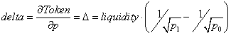
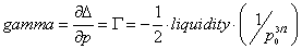
For the LP position, first, we start with the delta. The LP’s delta will change via a linear change in the reciprocal of the square root of the price:
The derivative of this with respect to price is the Gamma
So, the gamma for a pool position is pretty straightforward.
The gamma for an option can be calculated a couple of ways, identical for a call and a put. As we are replicating a straddle, we need to multiply this by 2.

[See here for a definition of these terms. Fun fact: Jimmy Wales’s first Wikipedia post was on the Black-Scholes model. This formula applies to one option, so the notional is the price. To generate the gamma for an arbitrary notional, we multiply this result by N/p, the number of options needed to generate a notional amount of N].
Option values, and their ‘greeks’ like gamma, are determined by the current price, volatility, time to expiration, notional, and strike. Only the current price is fixed, so this gives us an infinite combination of parameters to work with, but it’s helpful to assume the volatility is the asset’s historical volatility simply. Let us use 100% for ETH to make it simple (it’s probably about 85%, but close enough). Let us also use 1-month for the expiration, in that this is the most popular option maturity. This leaves us only with the notional and the strike. We can solve for these parameters a variety of hill-climbing methods, including the solver in excel.
Doing so generates the following comparison.
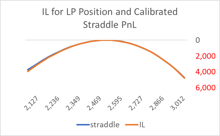
Even though I just targeted the gamma, the fit is almost perfect over the distribution of prices that span a day’s potential price movement. In this case, the straddle value is $21k, and the theta, or daily time decay, is $342.
For the option, the theta is calculated via
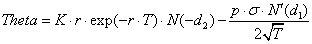
An option position’s theta must equal the cost of the IL via arbitrage, as proven by Black-Scholes
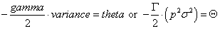
So, in this case, the LP’s gamma at p=2500, and liquidity=10,000, is -0.04. The one-day variance is 2500^2*(100%^2)/365=$17,123, so the theta derived from the LP position is $342.
Alternatively, one can apply probabilities to the pool IL losses over a day, generating $345 (off slightly due to approximation errors).
The bottom line is that this $1MM pool position bleeds $342 a day, which can be calculated in several ways. This adds up to a 12.5% loss over a year.
We can apply this to two of the most popular Uniswap pools, the ETH-USDC 0.05% pool, and the higher fee instantiation, the 0.3% pool. The revenue for LPs is just daily USD traded times the fee amount (0.05% and 0.3%). The cost is derived via the gamma (a function of liquidity, price, and volatility). We can pull the liquidity and price, and for the volatility, I pulled the 15-minute returns throughout the day (24 times 4 or 96 observations) to get the daily variance. Average daily liquidity encountered by trades, and the daily volume traded for these pools, can be pulled from places like Dune.
Uniswap data on USDC-ETH pools.

This table shows a persistent LP loss, with revenues around 80% of costs. This estimate is consistent with the results by TopazeBlue/Bancor earlier this year (see p.25), though that paper emphasized that ‘half of the LP providers’ lost money. This assumes LPs did not hedge their positions. More importantly, this should not be a primary takeaway, as it implies that all one has to be is above average to make money as an LP. As everyone thinks they are above average, this is a reckless implication.
There is no way for an LP to make money off these pools, no trick to make negative gamma disappear. Either the fees need to increase, or the volume needs to grow. The effect of a fee increase is obvious, but for the volume, the issue is these pools need more noise traders. Noise traders are just looking for convenience as opposed to arbitrage. They offset each other because when people act randomly, some buy and some sell, not affecting the price much at any time. If these pools can get more noise traders, LPs could make profits while fees and volatility are the same.
Currently, a lot of naive LPs are giving away money to arbitrageurs.
No comments:
Post a Comment