|
| Michael Heiser |
Joe Rogan and Tucker Carlson mentioned demonic spirits in a recent podcast, and my first thought was that they need to look up Michael Heiser. He was an Old Testament scholar who spent his career examining how various ethereal spirits fit into our world. Heiser died from cancer last year but has a ton of material online, as he did a weekly podcast discussing bible topics, not limited to his niche focus on angels and demons (see an intro video here). It's too bad he died because he would make for an excellent podcast with Rogan, as he was an excellent communicator and enjoyed investigating UFOs, Ancient Aliens, and Zechariah Hitchens (he was generally skeptical but found it fun; see here). More recently, Tim Chaffey wrote a book on the Nephilim, so perhaps that's an alternative for one of them.
Most intellectuals find the idea of ethereal forces patently absurd, but this is just because they don't understand the assumptions of their naturalistic worldview. Everyone believes in unseen forces and miracles; religious people merely own it. Cosmologists rely on the multiverse's infinite universes to explain various fine-tuning, such as the cosmological constant and the initial entropy of the universe; they also believe in dark energy, dark matter, and inflation, though these forces cannot be observed directly or falsified in any way. Secular origin-of-life researcher Eugene Koonin uses the multiverse to overcome the many improbabilities required. These scientific theories are untestable, differing from pre-scientific theories only by replacing God with hypothetical fields and forces.
Burying miracles into assumptions does not make them any less miraculous. An infinite number of universes could easily explain Genesis (with Charleton Heston as God), that we are a hallucinating consciousness imagining life as we know it, or that we live in a simulation designed by an ancient effective altruist. The only ontological difference between religious and naturalistic miracles is that religious people assign their creator not just with personhood but one who defines absolute, objective morality. I find the Biblical virtues stand on their own as optimal praxis for personal and societal flourishing, but simple Bayesian logic implies I should defer my ethical judgments to my creator, given the knowledge disparity. The Bible, however, teaches that my view has been and always will be a minority take under the sun.
Spirit Beings Who Are Not God
If you believe in the New or Old Testament, you believe there is more than God is not the only being in the spiritual realm. There is not only the trinity, but angels Gabriel, Michael, and the fallen angel Lucifer. Hebrews 12:22 mentions' countless thousands of angels,' and Psalm 89 mentions a divine assembly that includes many heavenly spirits, among many other mentions. No Jew or Christian thinks this implies polytheism.
A big problem centers on one of the words for God in the Old Testament. The word elohim is used thousands of times in the Hebrew Bible, and it usually refers to the 'God Most High,' Yahweh, aka God. This has led many to think every use of the word elohim refers to God, which is simply incorrect. First, note that elohim is a word like deer or sheep that can be singular or plural. For example, in Psalm 82, we read.
Elohim presides in the divine assembly; He renders judgment in the midst of the elohim
The word elohim here has two referents: the first for God is singular, and the second is plural because God is 'in the midst of' them. Elohim is used thousands of times in the OT to denote the God (aka Yahweh), but also reference different ethereal beings.
The members of God’s council (Psa. 82:1, 6)
Gods and goddesses of other nations (Judg. 11:24; 1 Kgs. 11:33)
Demons (Hebrew: shedim—Deut. 32:17)
The deceased Samuel (1 Sam. 28:13)
Angels or the Angel of God (Gen. 35:7)
Elohim is just a word for spiritual beings, and these are often mentioned in the Old and New Testaments. God is an elohim, but he is also the Most High, as in Exo 15:11: "Who is like you among the elohim, Yahweh?" If He is most high, He has to be higher than something else.
Understanding many other spiritual beings are interacting with God helps us understand the phrase in Genesis 1 where God says, "Let us make man in our image," or when God says, "man has become like one of us in knowing good and evil." Ancient Hebrew did not have the majestic we or trinitarian phrases.1
This is an essential point because the existence of other elohim is commonly overlooked by Christians, and this obscures some profound truths. How else would one make sense of 1 Kings 11, where God is in heaven discussing what to do with Ahab:
Micaiah continued, "Therefore hear the word of the LORD: I saw the LORD sitting on His throne, and all the host of heaven standing by Him on His right and on His left.
And the LORD said, 'Who will entice Ahab to march up and fall at Ramoth-gilead?'
And one suggested this, and another that.
Then a spirit came forward, stood before the LORD, and said, 'I will entice him.'
'By what means?' asked the LORD.
And he replied, 'I will go out and be a lying spirit in the mouths of all his prophets.'
'You will surely entice him and prevail,' said the LORD. 'Go and do it.'
God does not have a personality disorder; he has a council of other ethereal beings, other elohim. He does not need these helpers any more than we need dogs, friends, or children: they bring us joy, but also problems. Humans can empathize because we were made in his image. Many other verses make no sense if God exists in the spiritual world with only his alter egos (the trinity).
Spirits go Bad
Many cannot fathom why a good and all-powerful Yahweh would create beings who become evil, and the answer generally focuses on the importance of free will, which is part of being made in the image of God. There is endless debate on free will, whether one believes in God or not. For example, the existence of evil given a good, all-powerful God is puzzling, but it's also difficult to imagine a world without evil; the word evil would lose its meaning, as well as its antonym, goodness. If they are inseparable, like two sides of a coin, is a world without good and evil better than one with them? One can speculate, but the bottom line is that elohim, like humans, can and do go bad, creating evil spirits that manipulate men.
There are three significant calamities in human history. The first is Adam and Eve's fall in the Garden of Eden, the only one most Christians recognize. However, two others get less attention: the rebellions that led to the flood and tower of Babel incident, which directly involved evil elohim. There are many more texts relating to these latter falls in the Qumran texts (aka Dead Sea Scrolls) than the incident with the apple, highlighting they should get more of our attention.
The backstory for God's decision to flood the earth is mentioned in Gen 6:2-4

"the sons of God saw that the daughters of man were attractive. And they took as their wives any they chose. Then the LORD said, "My Spirit shall not abide in man forever, for he is flesh: his days shall be 120 years."
The Nephilim were on the earth in those days—and afterward as well—when the sons of God had relations with the daughters of men. And they bore them children who became the mighty men of old, men of renown."
The sons of God, fallen elohim, impregnate human females, creating 'mighty men of renown,' the Nephilim, translated as giants in the Septuagint. The Nephilim are referenced in several places, including descriptions of figures like Goliath, the Anakim, King Og of Bashan, and the Canaanite "giants in the land" targeted by Joshua's conquests. Christians often interpret the 'sons of God' who fathered the Nephilim as just good Hebrews, who contrast with the unrighteous' daughters of men.' This makes little sense because their offspring were clearly different, not just in size, but in their capabilities. Why would a sinful-righteous human pairing create supermen? The acceleration of evil created by these half-breeds and their progeny was a travesty so evil Yahweh decided to eliminate most of humanity.
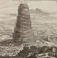
The flood did not fix the problem. A couple hundred years after the flood, there is the Babel incident, in which humanity attempts to build a tower to heaven, a rebellion based on hubris that offends God. In response, God not only disperses humanity into various nations, but he disinherits them as His people and puts them under the authority of lesser Elohim. This is recalled in Deuteronomy 32.
When the Most High gave the nations their inheritance, when He divided the sons of man, He set the boundaries of the peoples according to the number of the sons of God (Israel). But the LORD's portion is His people, Jacob His allotted inheritance. ~ Deu 32: 8-9
We know this refers to the Babel event because God apportions a table of 70 nations in Genesis 10 from Noah's three sons. In Genesis 11, after the judgment at Babel, each of these nations was assigned to a son of God, a lesser elohim, while one was kept for the Lord.
Historically, most Christians have read Deuteronomy 32 with 'sons of Israel' as opposed to 'sons of God.’ Currently, most English translations have Israel, but many have God, such as the ESV. While Israel is an accurate translation of the Hebrew Masoretic text used by Jerome, God was more common among Qumran texts and the Septuagint. This mistranslation led to a lack of interest in its implications, as in the ‘sons of Israel’ interpretation, one assigns rulers like Jacob, while in the ‘sons of God’ view, regional deities. The issue becomes prominent in Psalm 82.
Ps 82:1-2 Elohim presides in the divine assembly; He renders judgment in the midst of the elohim. How long will you judge unjustly and show partiality to the wicked? …
Ps 82: 6-7 I have said, 'You are elohim; you are all sons of the Most High.' But like mortals you will die, and like rulers you will fall.
God is not speaking to Jewish elders as elohim because humans do not sit in God's divine assembly (see Psalm 89 for a description of God's council). Further, it would make no sense to proclaim humans would die like mortals; they would have known that. Thus, Psalm 82 describes God judging the elohim he assigned to rule the nations, as described in Genesis 11 and Deuteronomy 32. You could easily miss it if you did not read 'sons of God' in Deu 32, which explains why this interpretation is relatively new (the Qumran texts that seal the inference were unavailable to Augustine, Calvin, etc.).
To recap, we have
Gen 6:2-4: Evil spiritual beings come down to earth, defiling women and creating a race of evil, mighty giants, the Nephilim
Deu 32:8-9: Recounts how God abandons 69 nations to lesser elohim but keeps one to himself that he would inherit through Abram.
Psalm 82: God condemns 69 elohim for being unrighteous rulers of their nations.
These are the types of dark forces that create problems for humanity.
The Watchers
The Book of Enoch (aka 1 Enoch) and The Book of Giants are prominent among the Qumran texts, and the expand upon the brief mentions above. Enoch refers to the sons of heaven as the Watchers. The Watchers see the daughters of men, desire them, and decide to come down from heaven and mate with them (as in Genesis 6). Their leader, Shemihazah, knows his plan is sinful, and he does not want to bear the responsibility alone, so the Watchers swear an oath on Mount Hermon, a classic conspiracy (they rebel against God, noted in Ps 82). The Watchers teach humans various 'magical' practices such as medicines, metallurgy, and the knowledge of constellations. This knowledge gives people great power but exacerbates their sin and suffering.
Enoch describes how the offspring of the Watchers and women became giants who dominated humanity, 'devouring the labor of all the children of men and men were unable to supply them.' 1 Enoch 15:8 refers to the offspring of the giants as demons. These beings are described as spiritual, following their fathers' nature; they do not eat, are not thirsty, and know no obstacles.
One might reject this description of an older form of Ancient Aliens click-bait. However, we can know this is true because listening to spirits is forbidden by God, which would make no sense if it were impossible.
You must not turn to mediums or spiritists; do not seek them out, or you will be defiled by them. I am the LORD your God. ~ Leviticus 19:31
While the Book of Enoch is not canonical, it should still be taken seriously. Both Peter and Jude not only quote from the Book of Enoch, but they quote the verses that directly describe the fallen elohim.2 Enoch is also quoted in 3 Maccabees, Ecclesiasticus, and the Book of Jubilees. It is favorably examined by the early Church fathers Justin Martyr, Irenaeus, Clement of Alexandria, Tertullian, and Origen.
A big reason Christians do not revere the Book of Enoch is that influential Christian Augustine ignored it. Augustine became a Christian as a Manichean who revered The Book of Enoch and emphasized the external battle of good vs. evil. Enoch's narrative does not mention human responsibility. It is a determinist view where evil originates from the deeds of the Watchers, in contrast to the Garden of Eden story, where sin emanates solely from our human nature. Ultimately, Augustine rejected Manichism; he thought our most pressing problem was the sin residing in all of us due to the initial fall of man in the Garden of Eden. Like many who fall away from an ideology, he tried to make a complete break as possible and dismissed the Watchers story.
Jesus and the Dark Spirits
This view of dark forces explains the cosmic geography mentioned in the New Testament.
To the intent that now unto the principalities and powers in heavenly places ~ Ephesians 3:10
against principalities, against powers, against the rulers of the darkness of this world, against spiritual wickedness in high places. ~ Ephesians 6:12
If you believe in the New Testament, you can't reject the assertion that demonic forces have a major role in human life.
The gospel's good news directly addresses the problem created by demonic forces. Christ enabled those under the lesser elohim's dominion to turn from those gods via faith. The breach caused by the Babel rebellion had been closed; the gap between all humanity and the true God had been bridged.
We see this in Acts, where Luke records Paul's speech in Athens. In talking about God's salvation plan, Paul says:
And God made from one man every nation of humanity to live on all the face of the earth, determining their fixed times and the fixed boundaries of their habitation, to search for God, if perhaps indeed they might feel around for Him and find Him. And indeed He is not far away from each one of us. ~ Acts 17:26-27
Paul clearly alludes to the situation with the nations produced by God's judgment at Babel, as described in Deuteronomy 32. Paul's rationale for his ministry to the Gentiles was that God intended to reclaim the nations to restore the original Edenic vision. Salvation was not only for the physical children of Abraham but for anyone who would believe (Gal. 3:28-29)
In Acts 2, the apostles, filled with the Holy Spirit, begin to speak in various tongues, allowing them to communicate the gospel to people from different nations visiting Jerusalem. Paul describes the disciples speaking in tongues as divided using the same Greek word (diamerizo) from the Septuagint in Deuteronomy 32, 'When the Most High divided the nations, when He scattered humankind, He fixed the boundaries of the nations.' Luke then describes the crowd, composed of Jews from all the nations, as confused, using the same Greek word (suncheo) used in the Septuagint version of the Babel story in Genesis 11: 'Come, let us go down and confuse their language there.' This mirroring highlighted that Jesus and the holy spirit would rectify the disinheritance at Babel and the subsequent oppression by corrupted elohim rulers.
Christ’s sacrifice gave people the ability to defy regional demons, but he did not eliminate them.
Demonic Ancient Aliens
In the Babylonian flood story, divine beings known as Apkallu possessed great knowledge, had sex with women, produced semi-divine offspring, and shared their supernatural knowledge with humanity. In contrast to the Bible, they were hailed as pre-flood cultural heroes, so Babylonian kings claimed to be descended from the Apkallus. To make the connection with Enoch even clearer, Apkallu idols were often buried in Babylonian house foundations for good luck, and were called 'watchers.' The Watchers relates to many mysteries, such as the discovery of bronze and iron or the creation of the pyramids. These demi-gods were presented as the good guys for many ancient Middle Eastern societies.
The ancient Greeks had their version of this, replacing Apkallu with Titans. These were regional semi-deities with knowledge from the gods that gave them great power. In Hesiod's Theogony, he mentions the titan semi-gods and how Prometheus stole fire from the Gods. Aeschylus's play Prometheus Bound describes the famous punishment for giving humans divine knowledge, as sinful humans would invariably use their greater knowledge to their ultimate detriment, the classic story of hubris. The takeaway here is that interacting with these demi-gods is a Faustian bargain.
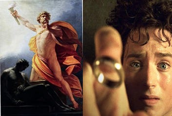
A common literary theme is to spin either the good Apkallu or bad Promethean interpretation of human development. For instance, in The Lord of the Rings, the ring has great power but ultimately destroys those who possess it; in The Godfather, Michael wins the war with the five families but loses his soul. In Percy Shelley's Prometheus Unbound and George Bernard Shaw's Back to Methuselah, knowledge from the gods generates human intellectual and spiritual development that brings humanity's eventual liberation and enlightenment through knowledge and moral improvement.
There is nothing wrong with technological improvement or efficiency. Bezalel is described as having great wisdom and craftsmanship and is promoted by God to create the first Tabernacle and the Ark of the Covenant. Noah was considered uniquely righteous and built a boat that could hold an entire zoo. The problem is succumbing to the temptations created by powerful, dark spiritual powers who know many valuable things that humans do not. Understandably, this power would seduce many. Any elohim who does this is contravening God's plan for their glory, which is evil. Many humans glom onto them, as they would rather rule in hell than serve in heaven, or just not care about the long run and prioritize the ephemeral pleasures of status and its spoils (‘eat, drink, and be merry for tomorrow we die’).
How demons interact with humans is unclear. As humans, we probably cannot exterminate them if we try, but we know we can and should resist them. There are many opportunities to aid and abet evil for a short-term advantage, but it is foolish to gain the whole world to lose your soul. While I doubt anyone can tell if someone is a demon puppet, let alone a demon, both have and do exist. We need not to be naïve and be wary. Discerning good and evil is difficult when dealing with fallen elohim, as they lie and are smarter than us. A simple rule is to speak truth to lies because God is truth. If you must lie to make your point, there's a good chance you are allying with dark forces.
see other 'us' language in Gen 1:26, Gen 3:22, Gen 11:7, Isaiah 6:8
1 Enoch 19:1 quoted in 2 Peter 2:4
For if God did not spare the angels when they sinned, but cast them into Tartarus
1 Enoch 1:9 quoted in Jude 14-15
It was also about these men that Enoch, in the seventh generation from Adam, prophesied, saying, “Behold, the Lord came with many thousands of His holy ones, to execute judgment upon all, and to convict all the ungodly of all their ungodly deeds which they have done in an ungodly way, and of all the harsh things which ungodly sinners have spoken against Him.