Uniswap version 3 (v3) uses restricted ranges, such as price ranges from $1000 to $2000 for ETH, while in version 2 (v2), the ranges are unrestricted (i.e., 0 to infinity). In v2, an LP supplies equal values of both tokens, while in v3, the relative values depend on the price bounds and the current price. LPs can choose a variety of price bounds called ticks. The LP ranges are defined by these ticks, one low and one high, bounding the LP’s range.
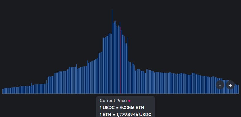
A current aggregation of v3 concentrated ranges for the ETH-USDC 0.3% pool
I will assume a simple ETH/USDC pool for the rest of this example, as opposed to tokens A and B. This makes it easier to interpret and is straightforward to generalize.
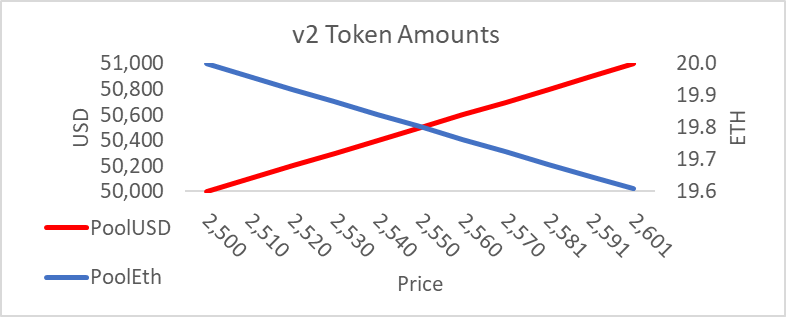
Within any set of ticks, there is a measure of pool liquidity called ‘liquidity’ in the Uniswap documentation. While this term has an intuitive meaning, it has a specific definition in the context of a constant product automated market maker (AMM).
To see how this is done, consider a v2 range defined over the prices {2500, 2601}, with a liquidity of 1000
Table 1
LP ETH and USDC, Liquidity=1000
ETH USD
ETHprice = 2500 20.00 50,000
ETHprice = 2601 19.61 51,000
Difference 0.39 1,000
Liquidity is more intuitive than its square, k, because it reflects how many dollars are needed to move the square root of the price by 1. In the above example, swapping $1000 USDC for ETH pushes the price down from 2601 to 2500, while buying $1000 would push the price up from 2500 to 2601. In v3, the trick is finding a way to replicate this price and quantity relation while not requiring all the capital in a v2 pool.
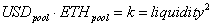
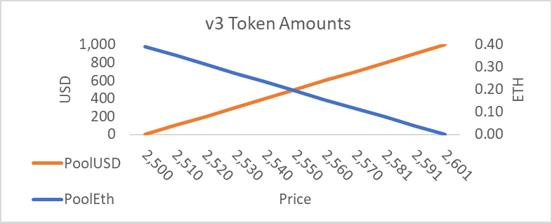
In v2, for a given amount of liquidity, USDC in the pool is always increasing with price, while ETH is continuously decreasing with the price. Their product at any given price is constant if LPs do not add or remove liquidity, and the pool is merely subject to trading. Below is a simple ETH/USD pool in the unrestricted range over a wide interval (0 to 2500).
Figure 1
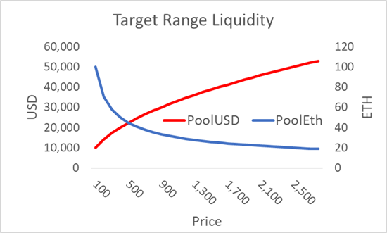
While v2 creates a nonlinear function for the token quantities over price, the relationship looks approximately linear within a range representing the average daily price change (~ 4%). If we constrain ourselves to the range 2500 to 2601, the pool amount of USDC spans from 50,000 to 51,000, while the ETH goes from 20.00 to 19.61. A concentrated range allows the LP to provide the net amount exchanged only in that range, not the extra USD and ETH needed outside that range. Thus, if the current price is 2500, and LP targeting the range {2500, 2601} needs only 0.39 ETH. She needs no USDC because she is only offering liquidity above the current price and does not have to provide USDC to buy; someone selling would push the price down and outside of her range, so that event is irrelevant to her. Similarly, if the price were 2601, she would only need to provide $1000 USDC and zero ETH.
Another way to see this is that in v2 and v3, within a particular set of ticks for a specific level of liquidity, the change in the pool tokens is identical; however, the amounts of tokens in these two contracts are not. Below in Figure 2, we see that in both cases, the changes in USDC and ETH are 1000 and 0.39, respectively, though v2 requires ten times the total amount.
Figure 2
To get the math to work with fewer tokens, we need to find the necessary adjustments to get the slopes of the above graphs to be the same because that represents the amount of ETH and USDC needed for price changes in this range. Let us call the amount of ETH in a v3 concentrated range ETHv3; this is the real or non-negative amount of ETH needed to satisfy traders within this restricted range. To match the v2 mathematics, we will call ‘virtual’ ETH, the ETH amount required to make the math work.
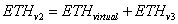
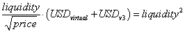
Starting from the standard v2 logic
We replace the ETHv2 with the new ETHv3 components
Substituting, we get
Given

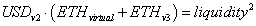
We can substitute for USD and get

Rearranging we get
The amount of ETH required for the v3 LP at the top of the range is zero, so we know:
The above equations imply that for the range {2500, 2601}, our virtual ETH is just
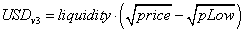
If the price goes above 2601, Alice is unaffected. That is because she is no longer providing any more ETH for USD. This implies that ETH-virtual over the entire price range is a function of the price at the top of the range. So now we take the definition of v3 compared to v2:

Given the equation above and generalizing by replacing 2601 with pHigh, we can solve for the ETHv3 for various prices within Alice’s range
This formula, derived from v2 pool math, gives us the accounting trick needed for an LP supplying concentrated liquidity on a v3 pool.
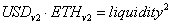
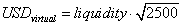
Similarly, we can apply the same logic to get the amount of USDvirtual within a given range:

Given the equation above, we can calculate the USDvirtual needed to make the v3 math work. Here the USDvirtual is a function of the lower price bound.

The v3 LP token quantities, their ‘real’ amounts, are adjusted by constants to match v2. As constants, they do not affect how price changes affect changes in the v3’s tokens within a range.
Range Math Outside the Range
Outside of the range, we need to make substitutions for the fact that the range is inactive; it does not supply liquidity outside the range. The LP has a simple position of {ETH=0.31, USDC=0} at and below 2500, and {ETH=0, USDC=$1000} at and above 2601. Thus, a concentrated range LP treats all prices above its range as if they were the price at the top of the range, and when below the range, the price can be treated as if it were the bottom price point.
One can use the following formula for a robust function within a program or spreadsheet:
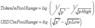
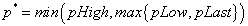
A v3 LP specifies {liquidity, pLow, pHigh} to establish a range. Combined with the current price, this implies a certain amount of USDC, ETH, and a specific USD value.
Tick Fee Math
A range of {2500, 2601} entitles the LP to a percent of the fee revenue generated from trades within that range. There needs to be a method for excluding trades below 2500 and above 2601. The accounting mechanism for doing this is extremely clever.
Each initialized tick is allocated a state variable for its ETH and USD fees. When combined with the global ETH and USD fee state, one can back out the fees generated to an LP, given their lower and upper ticks.
The tick fee allocation rule applies to fees for both tokens (here ETH and USDC), but we will focus on one token to simplify notation. Define globalETHfee as the global sum of the fees divided by the liquidity it experienced when applied (e.g., if the user paid $10 when liquidity was 1000, globalETHfee would increment by 0.01).
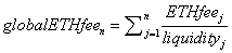
The equation above makes it easy to calculate an LP’s fee revenue. For an LP who provided liquidity at j=4, and assuming the current j=n, we would have

In v3, we must exclude the fees derived from trades outside the LP’s range. We use the following rules applied to all ticks to keep track of the relevant fee revenues for LPs with various tick endpoints. There are six different variables updated each time a tick is crossed. Relevant to the tick fee math, there is an ETH and USDC fee parameter for each tick. Remember that any LP range uses a subset of these ticks.
- If crossed for the first time
- tickFee= globalETHfee
- if crossed again
- newTickFee= globalETHfee - oldtickFee
- If above range, that is, pLast>pHigh
- tickFee(pHigh) - tickFee(pLow)
- If below range
- tickFee(pLow) - tickFee(pHigh)
- If in range
- globalETHfee - tickFee(pLow) - tickFee(pHigh)
The attached worksheet shows how this works for a range with pLow=1900 and pHigh=2000 and a fee of 0.3%. In columns G:H we see the per-trade fees, and in columns I:J we see the global state of the fees, which is just the cumulative sum. Columns K:L show how the tick fee state is updated on every cross for the 1900 tick, and columns M:N show how it is updated for the upper tick. This follows the ‘tick fee update’ rules above.
Columns S:T shows how the ‘fee calculation’ rule is applied at various prices—above, below, and within one’s range—using the global and tick fee state variables. In this example, I calculated fees for the {1900, 2000} range, which are in yellow. Note the LP here only should get fees for trades done in the yellow region. The “brute force” calculation method uses an excel if-rule to show that the logic generates the same results as counting all the fees generated in the yellow region (those are in columns g:h).
The pool generates a total of 281.34 in USDC and 0.097 ETH, and of this, in the end, 162.25 in USDC and 0.086 ETH go to the LP supplying liquidity from 1900 to 2000.
No comments:
Post a Comment