Spurious High Frequency Autocorrelation

 A curious aspect of high-frequency data is that most come from centralized limit order books (CLOBs) where the bid-ask spread makes the data look negatively autocorrelated as trades are randomly made at the bid and the ask.

The returns driving this pattern are well below transaction costs, so they do not generate an arbitrage opportunity. However, one might be tempted to use the high-frequency data to estimate variance for pricing options or convexity costs (aka impermanent loss, loss versus rebalancing). This is a problem because the 1-minute Gemini returns generate a variance estimate 40% higher than one derived from daily data.

Variance grows linearly over time; volatility grows with the square root of time. Thus for a standard stochastic process, the variance should be the same when divided by the frequency. If the return horizon is measured in minutes, the variance of the 5-minute return should be half of the variance of the 10-minute return, etc. Variance(ret(M minutes))/M should be constant for all M. It’s helpful to divide the data by a standard, which in my case is the variance of the 1-day return over this sample (1440 minutes), so we can clearly identify those frequencies where variance is over and under-estimated. If the ratio is above 1.0, this implies mean-reversion at this frequency (negative autocorrelation), and if below 1.0, this implies momentum (positive autocorrelation).

Here is the ratio of the m-minute return variance divided by m for various minutes, normalized by dividing by the 1-day return. It asymptotes to 1.0 at 300 minutes.

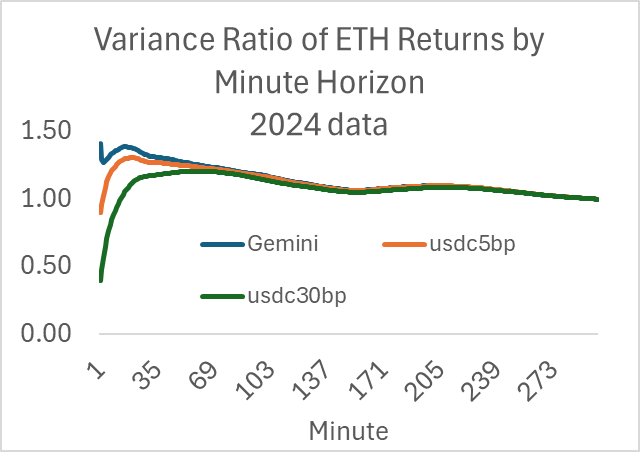
I added the ETH-USDC 5 and 30 bp pools, and we can see the effect of stasis created by the fee and lower transaction volume. The one-minute return variance ratios for AMMs are well below 1.0, implying momentum—positive autocorrelation—at that frequency. Again, the effect driving this is well below 5 basis points, so it’s not a pattern one can make money off.

A common and easy way to calculate variance is to grab the latest trade and update an exponentially weighted moving average. This would generate a variance estimate at an even higher frequency than once per minute. The perils of this are clear when many important data are linear in variance, such as the expected convexity cost, and 40% is big.

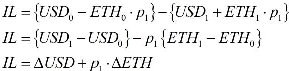
As a refresher, I show how the common concept for impermanent loss equaling a function linear in variance because it’s not obvious. We start with the original IL definition

This is measured as

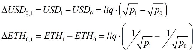
The following AMM formulas can substitute liquidity and prices into the above equation.

plugging these in, we can derive the following formula.

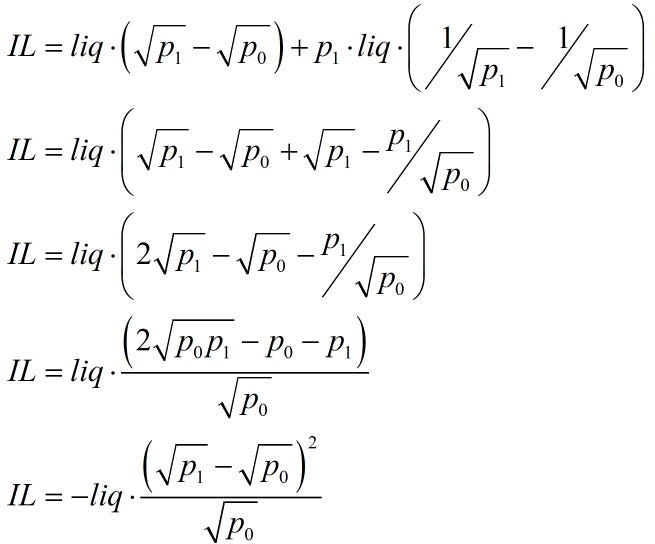
This ‘difference in the square roots squared’ function calculates a realized IL over a period (from 0 to 1). If one estimated this using daily data over several months, it would equal the expected IL via the law of large numbers.

One can estimate the expected IL using the expected variance and gamma of the position. The key nonlinear function on the AMM LP position is the square root of price, which has negative convexity. This implies a simple variance adjustment to the current square root to get the expected future square root.

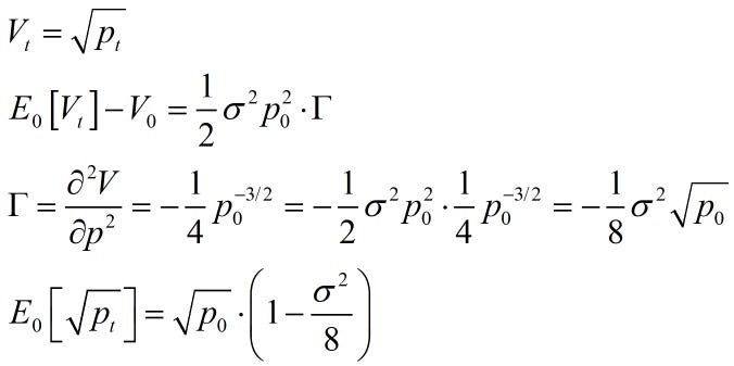
Note that in the above, the variance is for the time period from 0 to t, so if it’s an annualized variance applied to daily data, you would divide it by 365. Returning to the above IL formulated as a function of square roots, we can substitute for E[sqrt(p₁)] to see how this equals the ‘LVR’ equation with the variance.

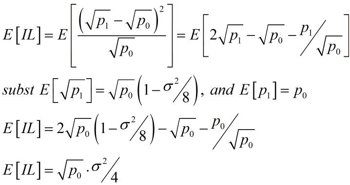
Using (p₁/p₀ - 1)² for the variance will generate the same formula as the difference in square roots squared if you use the same prices. We can’t measure expected returns, but average returns equal expected returns over time, and that’s all we have. One chooses some frequency to estimate the IL, regardless of the method. Just be careful not to use returns under a 300-minute horizon, as these will bias your estimate.