Tuesday, June 14, 2022

Why Slavery in the Bible Doesn't Bother Me

Slavery is often considered a shining example of how "the moral arc of the universe is long, but it bends towards justice." Many people cannot understand how a worldview, or a 'real' God, could have any legitimacy today if it ever tolerated such an institution. I am a Christian, and while I agree that slavery is abhorrent today, it was a moral advance in its time. Those asserting that ancient tribes should have condemned it categorically are just naïve prigs.

Ancients had no moral qualms over what we today would consider horrific crimes. Members of outside tribes were so different in language, religions, and manners that they were considered beyond the universe of obligation they applied to their own tribe. For example, in Homer's Iliad, King Agamemnon explains why Troy will be annihilated. 

"My dear Menelaus, why are you so wary of taking men's lives? Did the Trojans treat you as handsomely as that when they stayed in your house? No; we are not going to leave a single one of them alive, down to the babies in their mothers' wombs, not even they must live. The whole people must be wiped out of existence and none be left to think of them and shed a tear."

Genocide was not something anyone needed defending when dealing with vanquished foes. Ashoka the Great (280 BC) and Assyrian King Ashurnasirpal II (883 to 859 BC) boasted of genocide. When Rome razed Carthage in 46 BC, 150K Carthaginians were killed out of a total population of 200K to 400K. As late as 1850, the Comanche killed all adult males and babies in battles. When a tribe is at its Malthusian limit, its apologists will have no problem justifying such tactics.

Slavery or genocide was necessary because the survivors kept on fighting if released. For example, in 689 BC, the Assyrian King Sennacherib destroyed Babylon and carried a statue of their god Marduk back to Nineveh. By 612 BC, the Babylonians were strong enough to come back and destroy Nineveh, and the 2,000-year-old Assyrian kingdom never recovered. There were endless genocidal conflicts throughout the Bronze Age, so if a tribe, like the Hebrews, unilaterally chose to play nice and release captured soldiers, they would not have survived, and we would not even know about the Bible.

Unlike today, real existential crises existed all the time in ancient history. One of the worst genocides in human history happened in Britain and Ireland when invaders from Spain and France obliterated the natives around 2500 BC. This can be seen in that the frequency of the Y-chromosome G marker is now only about 1 percent, overtaken by those with the R1b marker, which makes up about 84% of Ireland's male population.

Around 2,500 BC, much of the European population's DNA was replaced with that of people from the steppe region near the Black and Caspian seas. This is a nice way of saying the men were killed. The Steppe Hypothesis holds that this group spread east into Asia and west into Europe at around the same time—and the current study shows that they made it to Iberia, too. Though 60 percent of the region's total DNA remained the same, the Y chromosomes of the inhabitants were almost entirely replaced by 2,000 BC. The history of humanity is not just the history of warfare but the genocides that accompanied it.

Slavery requires a society complex enough to have a formal justice system that enforces property rights, as highlighted by the many references to slavery in our oldest texts (Code of Hammurabi), law codes from 1700 to 2300 BC. It is an institution enforced not merely by the owner but by a community, as otherwise, enslaved people would run off at the first opportunity for a better life. Conquering tribes did not take the defeated men home and have them work as a group, they sold them off to individuals, diluting them sufficiently so that a slave uprising would be an impossible coordination task. Most people would prefer slavery to execution, however, making this a moral advance.

The feudal system applied to a continent united by a shared religion reduced the need for genocide or slavery in Europe. Serfs would serve their King regardless of which cousin won the job, and in either case, they would be allowed to worship the same god, so it did not matter too much. Yet the entire time, ethics were subject to prudential rationality. For example, ransoming captured nobility was financially prudent and honorable, but this principle was relaxed when costly, as all principles are. Thus, at the battle of Agincourt (1415), the English took so many prisoners that King Henry worried they might overpower their guards; he violated the rule of war by ordering the immediate execution of thousands. The selective application of principles in times of existential crises is rational and predictable (Cicero noted, "In times of war, laws fall silent.").

Prison is an invention of the early 1800s as an alternative to corporal punishment. Before that, jails existed merely to hold people until their trial, as no society could afford to house prisoners for a long time, which is why the death penalty was so prominent. As late as the 1700s, 222 crimes were punishable by death in Britain, including theft, cutting down a tree, and counterfeiting tax stamps. The alternatives, such as a fine or property forfeiture the average criminal did not have, and the non-punishment of criminals has never been an equilibrium. As Thomas Sowell has frequently noted, a policy must look at the trade-offs, not just the benefits, and these are often manifest in the alternatives.  

In Knowledge, Evolution, and Society, Hayek argued that intellectuals do not create morals; they grow and sustain themselves via natural selection. John Maynard Smith applied this reasoning to animal behavior. He outlined that a strategy must work as an evolutionarily stable strategy, which involves iterated games where payoffs affect the distribution of players in the next game.
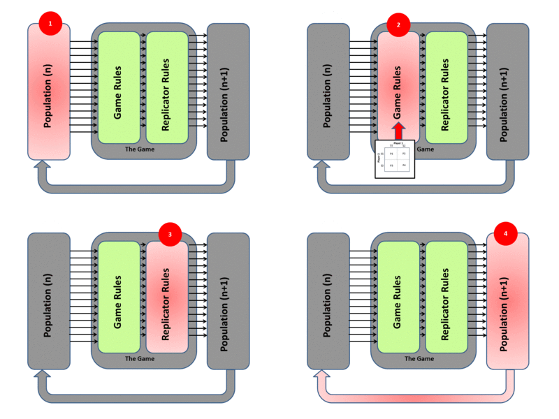
Evolutionary Game Theory

Mores, customs and laws must be consistent with strengthening the tribes that practice it, especially in the days when genocide was common. Productivity growth via social institutions like division of labor, or technologies like the plow, change the costs and benefits of human strategies. With more wealth, one can tolerate costs more easily, reducing the need for draconian punishment. This is a good argument for prioritizing policies that increase output over those targeting fanciful existential threats; wealthier societies can afford mores, customs, and laws that in a poor community would be irrelevant because they are infeasible.

The Bible laid the foundation for eliminating slavery once society could afford it. In the Bible, enslaved Christians are considered equal to their masters in moral worth (Gal. 3:28). Masters are to take care of their slaves, and slaves are encouraged to seek freedom (1 Cor. 7:21). In contrast, stoics of that time, like Seneca and Epictetus, never promoted manumission or the axiom that all men are made with equal moral status. They noted that slavers were also human, but this just implied slave owners should be nice to them, and Antebellum southerners were fond of quoting Seneca. The Philosophes of the 18th century, such as Rousseau or Kant, wrote almost nothing on the issue of slavery as practiced in their time.

The abolitionist movement only started in the late 18th century when English Christians (e.g., the Clapham Sect) and American Quakers began to question the morality of slavery. The principles underlying the condemnation of slavery revolve around the equality and dignity of all people. This was the primary motivational force of leading 18th Century British abolitionist William Wilberforce who viewed all people as "made in the image of God." This stands in contradiction to atheism which cannot justify nor defend the equality of humanity and its qualitative difference from any other sentient animal. While many Christians used the Bible to justify slavery, the more important point is that the seeds of slavery's eventual overthrow were based on Christian theology and championed by Christians, not secular philosophy and philosophers.

One can object to Christianity for many reasons, but it is ludicrous to suppose that slavery in the Bible proves it is morally bankrupt. If the Hebrews did not practice slavery, they either would have perished or had to have applied the viler tactic of genocide. If the first Christians campaigned for the immediate abolishment of slavery in an empire where 10-20% of the populace were slaves, the Roman government would have decimated them in the first century AD.

It is even more ludicrous to assert that because today's humanist intellectuals have never tolerated slavery, their worldview is morally superior to one based on a text written thousands of years ago that did. A mere century ago, humanist progressives were promoting colonialism, scientific racism, communist tyrannies, and fascism. Unlike slavery in the Bible, these were not the lesser evil policy given constraints of the time, but rather new policies foisted from above that increased human suffering and decreased human flourishing. To say that these errors were not 'real humanism' is special pleading.

Slavery was known in almost every ancient civilization. Outside of that sphere, slavery is rare among hunter-gatherer populations because it requires economic surpluses, the division of labor, and a high population density to be viable. Further, their social organization is too limited to create anything approaching a battalion, so they never engage in what one would call a war, and are thus never presented with the problem of what to do with one thousand enemy soldiers. 
Thursday, June 09, 2022

Uniswap LPs are Losing Money

[I'm posting these are Substack at efalken.substack.com, but I thought I post a couple here in case some people don't see those].

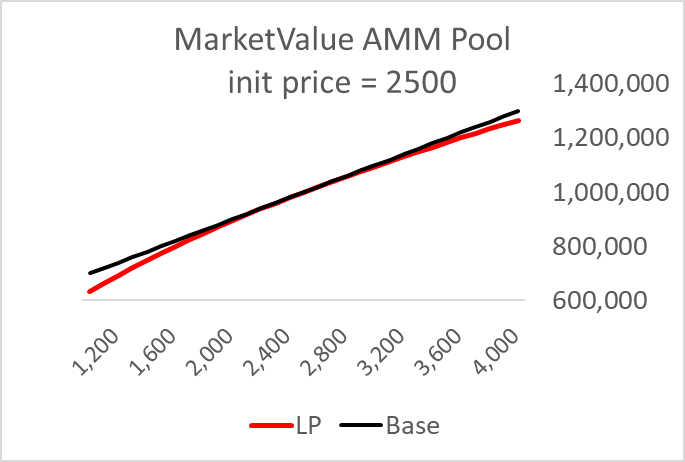
It is easy to ignore the option value when providing liquidity (LP for liquidity provider) because this is second-order relative to the risk from the price of one’s assets changing. Consider an unrestricted range where one provides $500k in ETH and USD at an initial price of $2500. The initial position is represented by the black line, the pool position by the red, and the impermanent loss (IL) is the difference between the two.

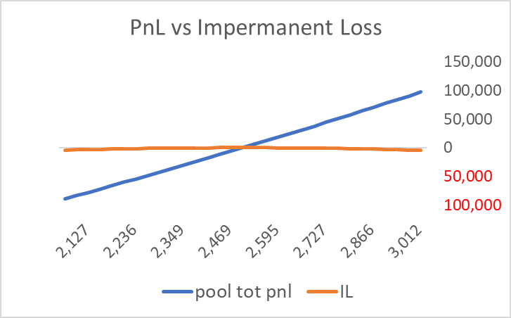
Another way to see this second-order distinction is by comparing that difference, the IL, with the pnl of the initial position. The orange line seems almost irrelevant. Almost.

It turns out that the IL will cost you around 12.5% annually for a token with a 100% annualized volatility (ETH’s vol is about 90%). Many people are being fleeced because they only look at the fee income in these pools.

The current automated market maker (AMM) LP situation is reminiscent of convertible bonds, where the seller of the bond includes an option for the buyer. If the stock price goes up, the bondholder can exchange his bond for a share of stock. As the value of this option is positive to the buyer, this lowers the bond issuer’s yield, seemingly saving the company money via a lower interest expense. Many ignorant Treasurers reasoned, “if the price goes up a lot, my shareholders will be happy, so they won’t be mad at me for some opportunity cost via dilution. If the price goes down, the shareholders will be happy because I saved the company money by selling a worthless option. Win-win!”

For decades convertible bonds were underpriced because their option value was undervalued, driven by the ignorant reasoning above. Savvy investors like financial wizard Ed Thorpe bought these bonds, and when hedged within a hedge fund, this strategy generated consistent Sharpe ratios near 2.0 without any beta through 2004. Eventually, investment banks became good at separating the options from these convertible bonds via derivatives, which made the value of the options within these bonds more transparent. Competition via arbitrage strategies pushed convertible bond prices up to accurately reflect the value of this option, and the days of easy alpha in convertible bonds were over.

An LP offers a pair of tokens for people to buy or sell at a current price. If you provide ETH and USDC to a pool, you implicitly offer a fixed price for buy or sale at every instant. In a limit order book, it would be analogous to offering to buy or sell Tesla at $750 when the current price is $750. If you leave that offer out there for a week, clearly, you will have bought only if the price went down and sold only if the price went up. This is called ‘adverse selection,’ because your offer selects the trade that is adverse to you.

Uniswap’s AMM isn’t exactly the same because the quantities offered do not have a fixed price, but the general idea is the same. It is like selling a put and a call at a fixed price, also known as a short straddle.

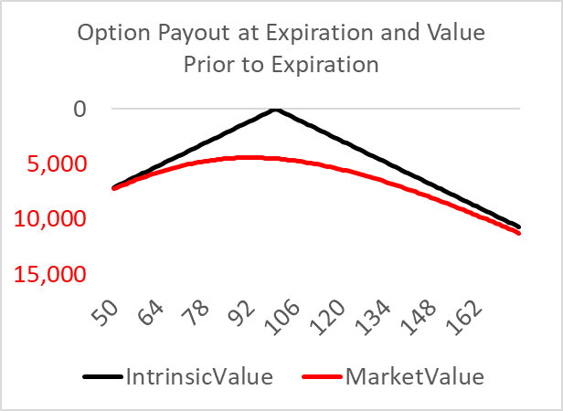
A short straddle payout looks like this:

The payout for a short straddle is strictly negative, but the option is sold for a positive amount. In equilibrium, the price should be slightly above the average payoff to compensate the seller for taking on risk, as potentially the seller could lose a lot of money. In contrast, the option buyer can only lose precisely as much as he paid. This risky nature of the option seller’s position is reflected in its convexity. The seller is exposed to negative convexity (second derivative negative) while the buy gets positive convexity. Positive convexity is like a lottery ticket; negative convexity is like asking The Godfather to do you a favor.

The cost of selling a straddle, or any payoff with convexity, can be calculated in two ways (see my earlier post here). One is by looking at the expected payoff of the option and discounting it with the risk-free rate. In the above graph, you would weight the points on the straight lines (intrinsic value) using a probability distribution given the time until expiration, current price, and expected volatility. This is the intuition behind the binomial options model. Another way is by calculating the convexity of the position, called ‘gamma,’ and multiplying it by the underlying price variance. This is the Black-Scholes method. One method assumes the seller does not dynamically hedge and one assumes the seller does, but that does not affect the value of the option sold, just the risk preferences or stupidity of the seller.

In application to providing liquidity in Uniswap, a good way to see the value of the options sold is by calibrating a straddle to replicate the pool position. In the attached spreadsheet, I present an ETH-USDC pool with an initial ETH price of $2500. The position was initially valued at $1MM and using the terminology of Uniswap, it has a liquidity=$10k (see my earlier post on how the term liquidity is used by Uniswap).

The IL for this position looks very much like a short straddle, so it seems fruitful to find the pool’s option analog. This is called the ‘replicating portfolio’ method of valuation. If you can replicate the payoffs of asset A with portfolio B, then they should have equal value via arbitrage. Here, the LP position value is

LP position = marketValue(liquidity=10k, p0=$2500)+IL

We know how to replicate and value the first term; it is just a $500k position in ETH and $500k in USD. So we need to find an option position that replicates the IL.

For the LP position, first, we start with the delta. The LP’s delta will change via a linear change in the reciprocal of the square root of the price:

The derivative of this with respect to price is the Gamma

So, the gamma for a pool position is pretty straightforward.

The gamma for an option can be calculated a couple of ways, identical for a call and a put. As we are replicating a straddle, we need to multiply this by 2.

[See here for a definition of these terms. Fun fact: Jimmy Wales’s first Wikipedia post was on the Black-Scholes model. This formula applies to one option, so the notional is the price. To generate the gamma for an arbitrary notional, we multiply this result by N/p, the number of options needed to generate a notional amount of N].

Option values, and their ‘greeks’ like gamma, are determined by the current price, volatility, time to expiration, notional, and strike. Only the current price is fixed, so this gives us an infinite combination of parameters to work with, but it’s helpful to assume the volatility is the asset’s historical volatility simply. Let us use 100% for ETH to make it simple (it’s probably about 85%, but close enough). Let us also use 1-month for the expiration, in that this is the most popular option maturity. This leaves us only with the notional and the strike. We can solve for these parameters with a variety of hill-climbing methods, including the solver in excel (see spreadsheet for this example).

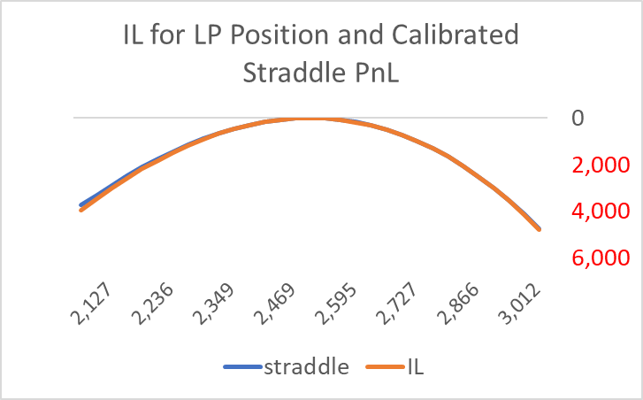
Doing so generates the following comparison.

Even though I just targeted the gamma, the fit is almost perfect over the distribution of prices that span a day’s potential price movement. In this case, the straddle value is $21k, and the theta, or daily time decay, is $342.

For the option, the theta is calculated via

An option position’s theta must equal the cost of the IL via arbitrage, as proven by Black-Scholes

So, in this case, the LP’s gamma at p=2500, and liquidity=10,000, is -0.04. The one-day variance is 2500^2*(100%^2)/365=$17,123, so the theta derived from the LP position is $342.

Alternatively, one can apply probabilities to the pool IL losses over a day, generating $345 (off slightly due to approximation errors).

The bottom line is that this $1MM pool position bleeds $342 a day, which can be calculated in several ways. This adds up to a 12.5% loss over a year.

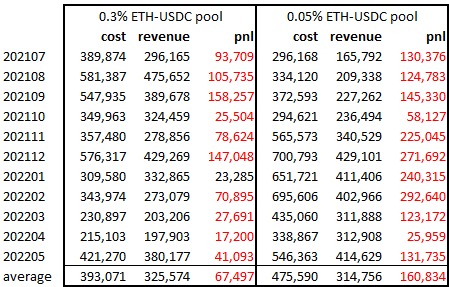
We can apply this to two of the most popular Uniswap pools, the ETH-USDC 0.05% pool, and the higher fee instantiation, the 0.3% pool. The revenue for LPs is just daily USD traded times the fee amount (0.05% and 0.3%). The cost is derived via the gamma (a function of liquidity, price, and volatility). We can pull the liquidity and price, and for the volatility, I pulled the 15-minute returns throughout the day (24 times 4 or 96 observations) to get the daily variance. Average daily liquidity encountered by trades, and the daily volume traded for these pools, can be pulled from places like Dune.

Uniswap data on USDC-ETH pools (downloadable spreadsheet ).

This table shows a persistent LP loss, with revenues around 80% of costs. This estimate is consistent with the results by TopazeBlue/Bancor earlier this year (see p.25), though that paper emphasized that ‘half of the LP providers’ lost money. This assumes LPs did not hedge their positions. More importantly, this should not be a primary takeaway, as it implies that all one has to be is above average to make money as an LP. As everyone thinks they are above average, this is a reckless implication.

There is no way for an LP to make money off these pools, no trick to make negative gamma disappear. Either the fees need to increase, or the volume needs to grow. The effect of a fee increase is obvious, but for the volume, the issue is these pools need more noise traders. Noise traders are just looking for convenience as opposed to arbitrage. They offset each other because when people act randomly, some buy and some sell, not affecting the price much at any time. If these pools can get more noise traders, LPs could make profits while fees and volatility are the same.

Currently, a lot of naive LPs are giving away money to arbitrageurs.

Tuesday, June 07, 2022

One-Month Trading Strategies

 About half of Robeco’s Quantitative Investing team recently published a short paper on monthly trading strategies (see Blitz et everybody Beyond Fama-French Factors: Alpha from Short-Term Signals Frequencies). I can imagine these guys talking about this stuff all the time, and someone finally says, “this would make a good paper!”

‘Short-Term’ refer to one-month trading horizons. Anything shorter than a month does not significantly overlap with standard quant factors like ‘value’ because they involve different databases: minute or even tick data, level 2 quotes. They are less scalable and involve more trading, making them more the province of hedge funds than large institutional funds. Alternatively, super-short-term patterns can be subsumed within the tactics of an execution desk, where any alpha would be reflected in lower transaction costs.

The paper analyzes the five well-known anomalies using the MSCI World database, which covers the top 2000 largest traded stocks in developed countries.

  1. Monthly mean-reversion. See Lehman (1988). A return in month t implies a low return in month t+1.

  2. Industry momentum. See Moskowitz and Grinblatt (1999). This motivates the authors to industry-adjust the returns in the mean-reversion anomaly mentioned above so it becomes more independent.

  3. Analyst earnings revisions over the past month. See based Van der Hart, Slagter, and van Dijk (2003). This signal uses the number of upward earnings revisions minus the number of downward earnings revisions divided by the total number of analysts over the past month. It is like industry momentum in that it implies investor underreaction.

  4. Seasonal same-month stock return. See Heston and Sadka (2008). This strategy is based on the idea that some stocks do well in specific months, like April.

  5. High one-month idiosyncratic volatility predicts low returns. See Ang, Hodrick, Xing, and Zhang (2006). This will generally be a long low-vol, short high-vol portfolio.

All of these anomalies initially documented gross excess monthly returns of around 1.5%, which, as expected, are now thought to be a third of that at best; at least they are not zero, as is the fate for most published anomalies.

Interestingly, Lehmann’s paper documented the negative weekly and monthly autocorrelation that underlay the profitable ‘pairs-trading’ strategy that flourished in the 1990s. Lo and Mackinlay also noted this pattern in 1988, though their focus was testing random walks, so you had to read between the lines to see the implication. DE Shaw made a lot of money trading this strategy back then, so perhaps Bezos funded Amazon with that strategy. A popular version of this was pairs trading, where for example, one would buy Coke and sell Pepsi if Coke went down while Pepsi was flat. Pairs trading became much less profitable around 2003, right after the internet bubble burst. However, this is a great example of an academic paper that proved valuable for those discerning enough to see its real value (note that Lehmann’s straightforward strategy was never a highly popular academic paper).

An aside on DE Shaw. While making tons of money off of this simple strategy, they did not tell anyone about it. They would tell interviewees they used neural nets, a concept like AI or machine-learning today: trendy and vague. I have witnessed this camouflage tactic firsthand several times, where a trader’s edge was x, but he would tell others something plausible unrelated to x. Invariably, the purported edge was more complicated and sophisticated than the real edge (e.g., “I use a Kalman filter to estimate latent high-frequency factors that generate dynamic alphas” vs. “I buy 50 losers and sell 50 winners every Monday using last week’s industry-adjusted returns”).

If each strategy generates a 0.5% monthly return, it is interesting to think about how well all of them do when combined. Below is a matrix of the correlation of the returns for these single strategies. You can see that by using an industry-adjusted return, the monthly mean-reversion signal becomes significantly negatively correlated with industry momentum. While I like the idea of reducing the direct offsetting effects (high industry returns —> go long; high returns —> go short), I am uncomfortable with how high the negative correlation is. In finance, large correlations among explanatory variables suggest redundancy and not efficient diversification.

STR=short-term mean reversion, IND_MOM=industry momentum, REV30D=analyst revision momentum, SEA_SAME=seasonal same month, iVOL=one-month idiosyncratic volatility.

Their multifactor approach normalizes their inputs into Winsorized z-scores and adds them up. This ‘normalize and add’ approach is a robust way to create a multifactor model when you do not have a strong theory (e.g., Fama-French factors vs Black-Scholes). Robyn Dawes made a case for this technique here. His paper was included in Kahneman, Slovic, and Tversky’s seminal Judgment under Uncertainty, a collection of essays on bias published in 1982. In contrast, multivariate regression weights (coefficients) will be influenced by the covariances among the factors as well as the correlation with the explanatory variable. These anomalies are known only for their correlation with future returns, not their correlations with each other. Thus, excluding their correlation effects ex ante is an efficient way of avoiding overfitting, in the same way that a linear regression restricts but dominates most other techniques (simple is smart). The key is to normalize the significant predictors into comparable units (e.g., z-scores, percentiles) and add them up.

I should note that famed factor quant Bob Haugen applied the more sophisticated regression approach to weighting factors in the early 2000s, and it was a mess. This is why I do not consider Haugen the OG of low vol investing. He was one of the first to note that low volatility was correlated with higher-than-average returns, but he buried that finding among a dozen other factors, each with several flavors. He sold my old firm Deephaven a set of 50 factors circa 2003 using rolling regressions, and the factor loading on low vol bounced from positive to negative; the model promoted historical returns of 20+% every year for the past 20 years, while never working while I saw it.

I am not categorically against weighting factors; I just think a simple ‘normalize and add’ approach is best for something like what Robeco does here, and in general one needs to be very thoughtful about restricting interaction effects (e.g., don’t just throw them into a machine learning algorithm).

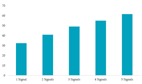
The paper documents the transaction costs that would make the strategy generate a zero return to handle this problem. This has the nice property of adjusting for the fact that some implementations have a lower turnover than others, so that aspect of the strategy is then included within the tests. The y-axis in the chart below represents the one-way transaction costs that would make the strategy generate a zero excess return. Combining signals almost doubles the returns, which makes sense. You should not expect an n-factor model to be n times better than a 1-factor model.

From Blitz et al

They note some straightforward exit rules that reduce turnover, and thus transaction costs, more than it lowers the top-line returns. Thus, in the chart below, no single anomaly can overcome its transaction costs, but a multifactor approach can. Further, you can make straightforward adjustments to entry and exit rules that increase the net return even while decreasing the gross return (far right vs. middle columns).

From Blitz et al

They also present data on the long-only implementation and find the gross excess return to fall by half, suggesting the results were not driven by the short side. This is important because it is difficult to get a complete historical dataset of short borrow costs, and many objectively bad stocks cannot be shorted at any rate.

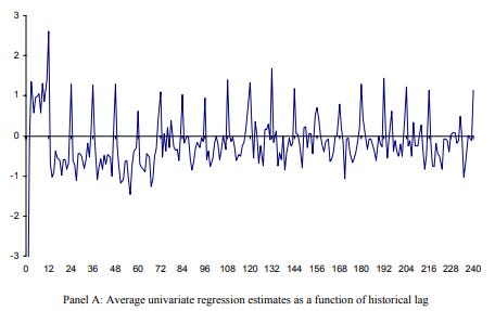
I am cautious about their results for a couple of reasons. First, consider the chart below from the Hesten and Sadka (2006) paper on the monthly seasonal effect. This shows the average lagged regression weighting on prior monthly returns for a single stock. Note the pronounced 12-month spike, as if a stock has a particular best month that persists for 20 years. The stability of this effect over time looks too persistent to be true, suggesting a measurement issue more than a real return.

From Hesten and Sadka (2006)

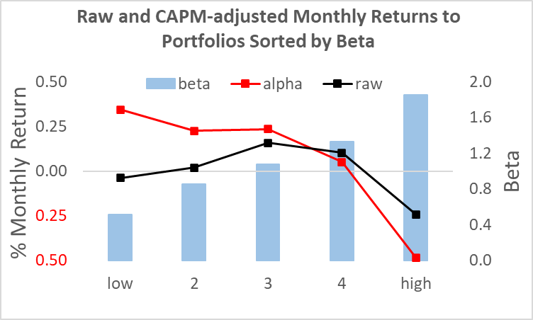
Another problem in this literature is that presenting the ‘alphas’ or residuals to a factor portfolio is often better thought of as a reflection of a misspecified model as opposed to an excess return. Note that the largest factor in these models is the CAPM beta. We know that beta is at best uncorrelated with cross-sectional returns. Thus, you can easily generate a large ‘excess return’ merely by defining this term relative to a prediction everyone knows has a systematic bias (i.e., high beta stocks should do better, but don’t). You could create a zero-beta portfolio, add it to a beta=1.0 portfolio and seemingly create a dominant portfolio, but that is not obvious. The time-varying idiosyncratic risk to these tilts does not diversify away and could reduce the Sharpe of a simple market portfolio.

US stocks presorted by CAPM beta, 2000-2020

Interestingly, Larry Swedroe recently discussed a paper by Medhat and Schmeling (2021). They found that monthly mean reversion only applies to low turnover stocks; for high turnover stocks, the effect is to find its opposite month-to-month momentum. I do not see that, but this highlights the many degrees of freedom in these studies. How do you define ‘excess’ returns? What is the size cut-off in your universe? What time period did you use? Did you include Japan (their stock market patterns are as weird as their TV game shows)?

Robeco’s paper provides a nice benchmark and outlines a straightforward composite strategy. If you are skeptical, you might simply add them to your entry and exit rules.