When investors are exposed to options, the hope is that somehow the exposure can be hedged without cost. This delusion is especially pernicious because it promotes the mistaken belief that somehow, a protocol can eliminate these costs via 'volatility arbitrage' or hedging. More importantly, understanding the hedging costs allows one to evaluate better the profitability of providing liquidity to automated market-maker (AMM) pools.
The essence of an option is convexity, a payoff that is a nonlinear function of some underlying price. Convexity can be hedged, but this just shifts the payoffs around; it doesn't reduce the expected cost of this option. This cost is independent of any transaction costs involved in hedging via the bid-ask, fees, or price impact. However, hedging is popular because it decreases indirect costs. A hedged position requires less capital, and capital has an interest expense (unless you are a G-7 country selling your bonds to your central bank). Further, people do not like risk per se, and almost everyone would take the certain expense of -2 over the crappy lottery where one gets either -12 or +10.
The nice thing about option theory is that you can prove things in many different ways. This is true for most mathematically derived results, such as how there are 17 ways to prove the Pythagorean theorem. The benefit of additional proofs is that, given our minds are different, one proof might appear more intuitive than the others for quirky reasons.
My point is the following: The expected loss of an unhedged short option position is equal to that of a hedged short option position. Further, as the cost of a hedge can be estimated much more precisely using volatility than a specific return over a long time period, one should use gamma and volatility to assess liquidity provider profitability as opposed to looking at how much a liquidity provider made over the past.
It is important to clarify a semantic point on expected returns. Expected returns for an individual are a constant; actual returns are a constant because they refer to the past and are unchanging; expected returns are a weighted average of potential actual returns. When I say the expected loss is the same, that means their number is the same, though they can be different in their distribution. For example, equal expected returns could be from a 100% weighting on one state, of the weighted average of two very different states.
Consider the binomial option pricing model (Cox, Ross, Rubinstein 1979). The basic idea is to create a riskless portfolio using a combination of a stock, bond, and option to a simple tree of states. This allows you to derive Black-Scholes with simple algebra, so it is the best way to teach someone about option pricing if they know nothing about it. I will not derive this model, just apply it.
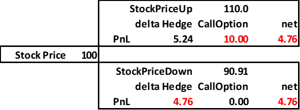
Assume a call with a strike of 100 and an initial stock price of 100; it will go up or down by 10%., and the riskless rate is zero. This implies the following future state space:

The above parameters for calculating the probability of an up and down move ensure the expected return equals the risk-free rate, which is what we want. In practice you need to get the up and down state values correct, and use many periods, but the gist of this approach falls out of a simple one-step model.
The portfolio is riskless if you hedge this with a stock position equal to the call's delta. In the binomial model, you can calculate a call option’s hedge exactly with the simple formula
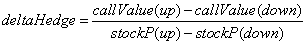
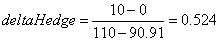
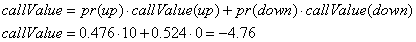
Given a delta of 0.524, this implies the call writer hedges by shorting precisely this amount of stock. The result is to generate the same payoff, whatever happens, -4.76.
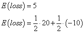
Note that the expected value of the call option is just the probabilities times the final value
While the call value is the same using either the binomial model or just present valuing the call liability, note that in the latter case, the seller would experience an expected loss of 10 in one state and 0 in another. In the hedged case, it would be the probabilistic average for certain. Hedging does not change the expected loss for someone selling options; it just makes the expected loss less variable.
Another way to see why there is an unavoidable cost of convexity, consider the case of a straddle, which is the combination of a put and a call with the same strike. In this example, your initial delta is approximately zero, with the positive call delta offset by the negative put delta. However, once this straddle moves, the deltas change, implying a hedge.
Consider a straddle with a strike of 100, and it can move up 1.1 or down by 1/1.1. The price tree over two periods and the corresponding straddle intrinsic value would look like this:

The above prices imply the following straddle payoffs:
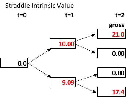
Given the tree parameters, we see that the delta becomes either +1 or -1 at step time=1 so that a hedge can be applied at time 1. This would then hedge the final period payoff. Note if we add this hedge pnl to the final pnl from the straddle, we get a much more precise loss, as opposed to the more bimodal one in the unhedged case.
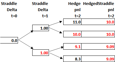
Here it is clear that the cost of the hedge comes from the fact that the initial delta is off once the first state is revealed, and you cannot do anything about that. This is a dynamic hedge, unlike the static hedge in the earlier example, but the result is the same in that the expected loss (-9.52) is exactly the same.
Another way to see this is by using a simple derivative. Consider the case where one hedges a derivative valued at p^2. This derivative would be a very inefficient mechanism for generating convexity, which is why active options markets use strike prices instead of 'square' prices, but it makes for a simple example.
The delta of this derivative is 2*p, so a seller of this option would hedge it by going short 2*p units. If p=10, the initial value of the squared derivative would be 100, and the seller would hedge by shorting 20 units. The net payoff space would then be as follows:

Note the expected loss of this squared derivative is -1, the average of +19 and -21. The hedged portfolio can make this expected loss certain, but it does not change this value.
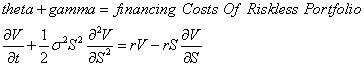
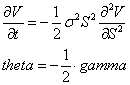
A final way to see that hedging costs are inherent in options is via continuous-time mathematics. The Black-Scholes option formula was derived via a dynamic hedging argument. The hedge replicated the valuation of the call option, creating a riskless portfolio. In the Black-Scholes PDE below, V is the option value, S the stock price, r the risk-free interest rate, and s (sigma) the volatility.
The equation shows the option's time decay (theta) plus its convexity return (gamma) equals the riskless return from a long position in the derivative and a short position and a hedged amount (dV/dS shares) of the underlying.
The solution to the partial differential equation when you add the boundary conditions (e.g., V=max(S-K,0)) is the familiar Black-Scholes model. More importantly, given we know this equals the binomial model, with its clunky steps, this proves that hedging more frequently does not change the direct hedging costs (i.e., expected loss). This dynamic replication approach assumes zero transaction costs and hedges incrementally at the slightest step imaginable. Even if you could trade your hedge at the mid-price every second, you would still generate the same expected loss as you would with a discrete set of 2 periods, or in the case where you did not hedge.
More interestingly, the cost of convexity here is put into a rate, which is called theta. If we assume the right-hand side of the above equation (the financing) is zero (because the riskless rate r is zero), we can see the relationship between theta and gamma. Theta is the expected time decay of the option price, but one can think of it as a funding rate or a fee rate.
If you know the gamma, you will know how much a fair amount of revenue would be. In the Black-Scholes model, one assumes the value of the option must be such that the hedging cost, -½*gamma, must equal the theta for an equilibrium. If theta were too high, no one would buy the option, and no one would sell it if they were too low. The nice thing here is that estimating gamma is pretty straightforward, as you just need the price and volatility.
In Uniswap liquidity pools, many liquidity providers look at the fee income as pure revenue, ignoring the value of the option they have written. This is easy to do because the option is not exactly like your standard option, but instead is this strange basket of coins. That mental block is a bigger subject than I can address here, but the bottom line is that this cost is present whether you calculate it or not, similar to how your car depreciation is costing you even if you don't think about it.
More importantly, the cost of providing liquidity is poorly measured by taking the price path over the past year and seeing if certain option sellers made or lost money. One should assume the sellers were hedging, whether they were or not. If you merely look at the price path, then a move from 100 to 200 to 100 will show LPs making a lot of money, while a price path of 100 to 200 to 300 would show LPs losing a lot of money. This method is like taking the annual return as an estimate of the stock market's volatility over that year. If you are analyzing whether or not to become an LP, this is a horrible way to do it.
People should use volatilities to estimate the hedging or gamma costs of providing liquidity in AMM pools.
No comments:
Post a Comment