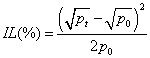
Falkenblog: A Simpler Formula for Impermanent Loss

There are many articles on impermanent loss, and most present an explanation where a formula is alluded to in many words but never presented (see here, here, here, and here). To cut to the chase, the Impermanent Loss for an unrestricted Uniswap liquidity pool can be calculated as

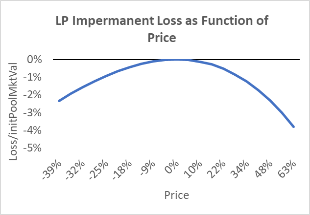
This is a unitless measure in that it represents the Impermanent Loss as a percent of the initial investment value, in that the graph below is identical regardless of whether your initial price is 1.0 or 100, or whether you put in $7 or $777. If you put in $100 of tokens, the formula above tells you that you would lose $2.34 if the price fell 39%, as shown in the chart below.

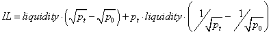
I found two articles online with formulas, but they require the user to read a bunch of words to figure out how to apply them. For example, Peteris Erins presents the formula:

eq2

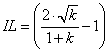
I find this formulation annoying because in the Uniswap v3 white paper k is liquidity^2, while here it is the gross return, pt/p0. Further, you are assumed to know this should be multiplied by the initial token quantities at the current price.

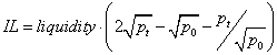
Another common online formula can be found in the oft-referenced study of LP impermanent loss by TopazeBlue, which presents the IL as

eq3

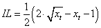
They make it unnecessarily complicated by defining xt as the ‘exchange ratio normalized so that x0=1,’ as opposed to defining it as the gross return (i.e., pt/p0). Their number applies to the initial pool investment as mine does.

I like my formula because it makes the pnl distribution more intuitive: it’s proportional to the square of the difference in starting and ending square root of price. Further, it is obvious how the LP’s loss is symmetric and negative, analogous to a short straddle position. Plus, I don’t add new letters like x or k!1

All three give identical results, however, so, use whatever works for you.

For anyone interested, it can be derived in two ways:

Derivation 1

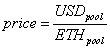
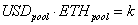
Everything comes out of a couple of equations. First, the price is represented by the ratio of the tokens in the pool. For example, with 2500 USD stable coins and 1 ETH, the price would be 2500, which is just common sense.

eq4

Secondly, for an existing pool, a trade with ETH going in and USD going out is subject to the following rule: the product of both tokens must be maintained at its existing level, a constant we will call k.

eq5

The two above equations are the basis for calculating changes in price or tokens as a function of other variables. Any change in USD or ETH must satisfy the following equation so that the product of the two tokens remains constant:

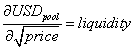
k will vary for a given price as liquidity is added and removed. For example, with {USD, ETH} equal to {2500, 1}, k=2500, while if it were {5000, 2}, k=10000. We define liquidity as the square root of k, the geometric mean of the tokens in the pool. This metric is more meaningful (see below), so we will replace k using the definition

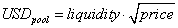
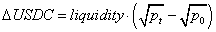
Given liquidity and price, we can derive the amount of USD in the pool. We do this by combining eq4 and eq5 to get

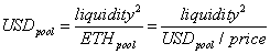
Which simplifies to

eq6

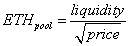
Similar math applied to ETH gives the equation for ETH as a function of liquidity and price:

eq7

Change in price and change in tokens

Given eq6 and eq7, a change in tokens is simply the difference in the quantities computed at an initial price (p0) and an ending price (pt):

eq8

eq9

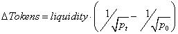
Here we see that liquidity represents the number of dollars exchanged for every integer change in the square root of price. This is why liquidity is more intuitively meaningful than k.

Fill price as geometric mean

Unlike centralized limit order books, a nontrivial order will not take out a singular price listed by a limit order, but traverse a continuum of prices based on the above axioms. This makes the fill price a little trickier. The fill price (pFill) is defined as the ratio of the USD and tokens exchanged in the trade.

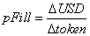
Substituting with eq8 and eq9 we get

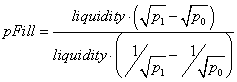
This simplifies via standard algebra to the geometric mean of p1 and p0. This fill price formula allows us to get better intuition as to token amounts in ranges.

While the above does not work if p1=p0 (division by zero), in that case, the fill price is trivially p1 or p0.

The LP’s profit as a function of the starting and ending price of a transaction is the number of tokens bought/sold times the difference in the current (or ending) price and the fill price.

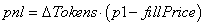
substituting we get

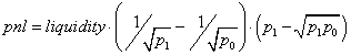
simplifying we get

eq11

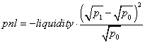
Now, here I’m using p1 instead of pt, but this applies to the cumulative change from p0 to pt as well. It’s more intuitive to think about as a single transaction, but whether one gets to pt via one transaction, or 27 transactions with buys and sells, the result is the same.

Note also I’m calling it the LP’s pnl, as opposed to the LP’s IL. This is because the LP is taking the other side of a trade that is pushing the price, and necessarily loses money the further the final price is pushed from the initial price. If the LP borrowed ETH to initiate his pool position, this would be his USD pnl; if he had the ETH initially, it would be an opportunity cost. In either case, it represents what is generally known as the IL.

If the price were USD/ETH, this would be denominated in USD. To turn it into a percent of the initial investment, we need to divide it by the initial investment. The USD value of the initial investment is just 2 times the value of the USD initial investment since the ETH initial investment value equals the USD initial investment. By substitution of eq6, our initial market value sent to the pool is then a function of liquidity and the initial price:

eq12

Dividing eq11 by eq12, we get the loss in percentage terms for the LP given a starting and ending price.

Derivation 2

The IL in USD for an ETH-USD pool is the value of the current pool position compared to the initial quantities at the current price.

rearranging we get this in the change in tokens

We can substitute for the change in USDC and ETH tokens using functions of liquidity, and starting and ending price. Note we always use the square root of price, which is why this is a state variable in Uniswap pools. Using eq8 and eq9, and substituting we get: