Panoptic received $11.5MM in VC funding, and now Uniswap is providing them with some reward money (1 billion Panoptic Incentive Points available!).1 Many hope that extensions like Panoptic that build upon automated market makers (AMMs) will solve the AMM liquidity provider (LP) unprofitability problem by encouraging LPs to remove liquidity and transfer the implicit option they are selling to explicit option buyers [see Part 1 analysis here].
The basic Panoptic premise is that since the value of an option's premium is based on its gamma, a measure of convexity, the gamma within LP positions can be used to create an array of options: puts, calls, and various combinations thereof. If the Uniswap LP position gamma is rewarded correctly, the fee revenue equals the convexity costs, and the gamma can be sliced and diced into virtually any option combo imaginable. This eliminates the need for an oracle or limit order book, both of which are especially difficult for options because these derivatives are more prone to adverse selection, as a 0.1% ETH price movement generates a 1.0% price movement on an at-the-money 7-day option. Standard tradFi options have higher spreads than their underlying assets for this reason, and they have micro-second latency compared to at least a second on the fastest decentralized blockchains. I can see why many find it potentially promising.
Many things work in theory but not in practice: macroeconomics, socialism, wind farms. It takes a lot of work to understand essential details, and most people are comfortable with a vision if they have no reason to doubt its plausibility. At this early stage of defi, developers and VCs cannot ignore the details. For me, Augur is the archetype of a simple idea that seemed attractive, but when you looked at their mechanism for offering and taking bets in the context of Ethereum's gas costs, you could see it was doomed. I will try to make clear why their approach needs radical refocusing to have any chance of working. Their out-of-the-money options are profoundly different than standard out-of-the-money options, and I do not see a market there. Their in-the-money ranges can replicate straddles, but their matching and pricing mechanism makes me think selling actual straddles using Uniswap as an oracle would work better.
To see the problems in Panoptic’s approach, it is helpful to compare it to standard options.
Standard Options: Unhedged
A naïve option seller collects a premium and hopes the option expires worthless. The intrinsic value of an option is the value of the option if it were exercised instantly, and the option premium above the intrinsic value reflects the seller's convexity cost. Option sellers have negative gamma, also called negative convexity, while buyers have positive gamma. The expected value of a payoff with positive convexity is greater than its current value, and this difference is the option's time value.
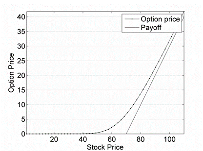
The real innovation in Black-Scholes was proving this option premium is simply the expected value of the option using the risk-free rate, which removes the subjective expectations from the problem. One assumes the underlying will increase at the risk-free rate, so all one needs is the maturity, underlying price, and a volatility estimate.

The short call option PnL below shows the positive payout below the strike price of $3800, representing the option's price (premium) received at instantiation by the seller. Above the strike, the PnL declines linearly.

Standard Options: Hedged
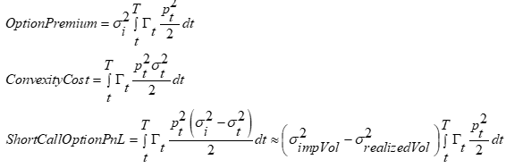
Professional market makers hedge to reduce their pnl variability, which reduces their capital costs and makes it easier to see if one's protocol is truly profitable (knowing you aren't making a profit is better learned early). By delta hedging, one can transform the option payout into an expense with a much lower variance. In an efficient market, an option's time premium equals the convexity costs incurred while delta hedging on average (there's a vega premium in standard equities, but we'll ignore that here). An option's implied volatility is the annualized volatility implicit in the option price; a number like 65% implies a 1-standard deviation log return over the next year is 65%. In a standard call or put option, the option premium is linearly related to an option's variance, which is the volatility squared. Still, it's hard to get intuition on variances, so we think about volatilities and apply them as variances in option pricing formulas.
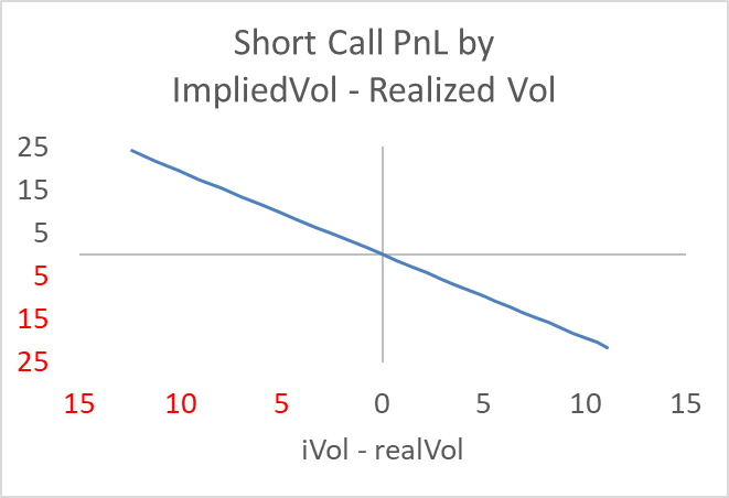
Ultimately, the bet for a hedged option seller is that the implied volatility is greater than the realized volatility. Given an option model, one can transmogrify implied vol into a price and vice versa, and so options are traded on price in an accounting sense but trade on vol in a trader's head. If the implied is 65%, and the realized is 60%, the hedged seller makes money regardless of the ending price; if the realized is 70%, the hedged seller loses money.
For a hedged seller, one can ignore everything and focus on the implied and expected vol. As in standard trading, one hopes to sell slightly above and buy slightly below the expected realized volatility. While ideally, one sells as much as one buys for each option (strike, maturity, etc.), the residual net position implies a delta hedging algorithm that can be automated. This leaves the standard option subject to risk if realized volatility is much higher than forecast, but an options market maker can hedge their net volatility risk generated by the overall market via a liquid option position in a market proxy and thus only be exposed to idiosyncratic risk. For a large options trading firm, idiosyncratic risks should cancel out.
Panoptic Options: Unhedged
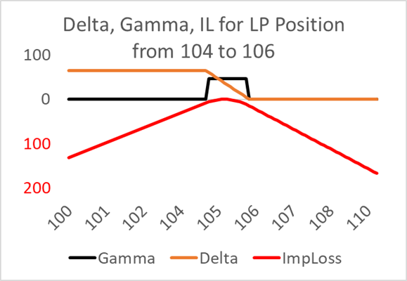
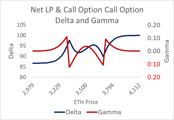
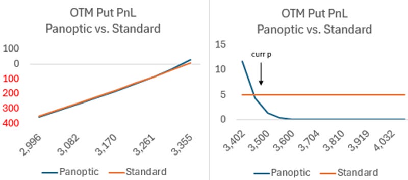
The unhedged Panoptic option is like a short out-of-the-money call and/or put, but unlike standard options, there's a significant price range where the gamma is zero. When the gamma is zero, the position has a 0.0 delta if the range is below the current price or 1.0 if the LP's range is above the current price. This aspect of LP positions makes them unlike standard options, which have a non-zero gamma even when the option's strike is out-of-the-money. This is because an LP can exercise his option at any time, unlike in standard options, where only the buyer has the right to exercise the option. I will abstract from this non-option portion of the LP position as if it is hedged, so the unhedged LP position means the LP is not continuously adjusting his delta where his range is active. Ignoring it is helpful because this aspect of an LP position is both riskless and returnless.
An important thing to remember in financial modeling is the expected value of a portfolio is just the sum of the expected value of its constituents. This means every asset can be evaluated in isolation. Thus, looking at the LP's range in isolation, only if and when it is active, is sufficient for valuing it.
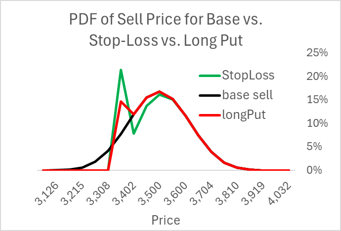
Panoptic prices their options using realized fees as opposed to an upfront premium. This makes the Panoptic options path-dependent. Consider the trinomial lattice below that moves through two trading periods. End prices generate the distribution used to calculate option prices, and these have the standard bell curve distribution around the starting price. Panoptic's model uses the fees generated in various ranges, assuming those fees reflect an implicit implied volatility to compensate for the convexity costs incurred. The distribution of this fee generation over the ending price distribution is leptokurtic—more peaked than a normal distribution—because earlier periods are biased towards the initial price. If we sum up the amount of time spent in various price ranges, this implies the price range's proportional contribution to expected convexity costs. Using a lattice, one can normalize the resulting sums to add up to 1.0, creating a standard probability distribution.

The graph below highlights the leptokurtic nature of the time spent in various ranges. The further the range is from the current price, the lower the probability range will be active, and this probability is significantly less than what is implied by the end price distribution.

An LP range may range from $3600 to $3700, and the time spent in that range is not apparent given the asset's starting and ending price. To see this, we can measure the ultimate end price distribution for all the prior periods where the range was active. One can do this using Monte Carlo simulations or a lattice. It's not super complicated, but going into detail would probably not interest most readers, so I will simply note that the end price distribution for out-of-the-money ranges is shifted to the left or right, where the relevant range is the peak of the distribution.

This means that if the current price is 3500, and the range is from 3800 to 3810, the fees generated by that range over time will get distributed in a normal distribution around that range across the end price. Most importantly, the further the range is from the ending price, the lower the probability the range was active.
This creates a PnL for out-of-the-money ranges that are zero the further the end price is from the range, as neither impermanent loss nor fees are generated. When the end price approaches the range, expected fees become positive and peak in the middle of the range, while the impermanent loss kicks in at the start of the range and accelerates to the end of the range. If the AMM is generating the requisite amount of fees, the expected value of this PnL is zero. This can be calculated by multiplying the various payouts by the relevant probabilities. This is similar to a standard out-of-the-money short call option, which has a large region where its PnL is positive and a smaller region where it is significantly negative.

The LP range PnL is a variant of the butterfly spread, where one pushes the further-out long call out to generate the asymmetric distribution we see in the out-of-the-money range. The trader presumably wants to cap their gamma exposure in the asymmetric butterfly and pays less for this by buying a further out-of-the-money call.
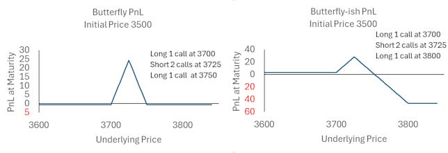
Butterflies are useful for estimating an implied volatility curve and understanding the current volatility skew. Butterfly spread traders usually target a specific strike because the implied vol on that strike is out-of-whack. Anomalous strike implieds can result from buyers anticipating a specific event, a case where fundamental information is not captured in a normal distribution. Traders who target these implied vol anomalies tend to trade the vol, hoping to sell later when the implied goes back to normal, meaning they are delta hedging their convexity. The unhedged out-of-the-money LP range does not have a good analog as an unhedged standard option, as unhedged option sellers are attracted to the certain premium revenue they hope will cost them zero.
Panoptic: Hedged Range
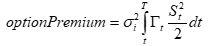
What about professionals or 'protail' option sellers? Starting with cost, we have the standard option convexity cost applied to ranges, which have

This generates the convexity cost function (aka theta)

Here, liquidity is zero outside the range, so the LP's convexity cost is only incurred within the range. The revenue function is also off outside the range. The trick here is to solve for an implied volatility using the range's gamma to equal the fee revenue. As the fees substitute for implied volatilities in ranges, there is an implied volatility one back out of the fee revenue.
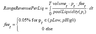
If the AMM is getting paid for its option expense, the convexity costs for this range equal the range revenue. We can put the revenue and cost together to get the total PnL

Since the total fees per unit of liquidity for a range are calculated in Uniswap's contract, we can use this number to generate a range implied vol.

We calculate the range's pnl by looking at the revenue minus the expense.
RangePnL = RangeFeeRevenue - RangeConvexityCost
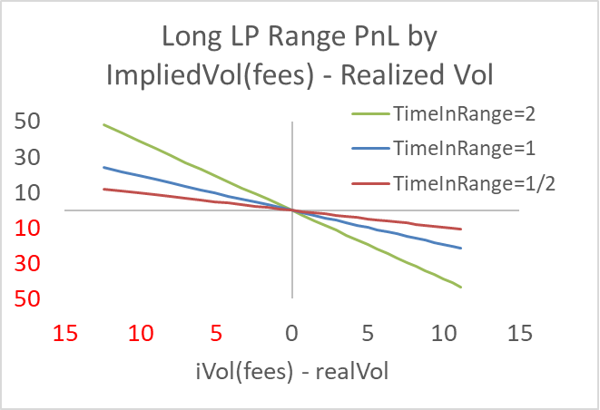
In terms of range implied and realized vol, is

This can be approximated by

The net result is then similar to the standard hedged short option PnL, except instead of using a known implied volatility, we have the range implied volatility, which is a function of the realized revenue (if any!) transformed into a volatility. Even if one knows the future trading volume, the fee revenue is shared pro-rata based on the pool's aggregate liquidity in the range, and there is considerable liquidity volatility over time. If the liquidity doubles, your fixed liquidity position's fee revenue halves. This year's daily liquidity volatilities for several AMM pools suggest this uncertainty is material.

The final big difference from the standard option is the path-dependent ‘time in range.’ This creates an orthogonal randomizing effect on the notional of the range pnl, as it can amplify a loss or a profit. A price can move way up and down, barely encountering the range it ultimately ends in; it could also stay in the range its entire life. This variable's resulting distribution is effectively uniform compared to a normal distribution. If you expect a number like 10, you probably will see a number like 5 or 20.
In Summary
The asymmetric butterfly spread is not popular among retail traders who do not hedge because out-of-the-money ranges generate little or no fee income if the price moves as retail option sellers expect. Locking up capital in a position that probably generates no revenue yet still generates a sizeable potential loss is something I can't imagine any option seller would find attractive.

For option sellers who hedge, the payoff is unattractive, but less so. The problem is that instead of betting on the realized volatility, one is betting on the difference between the realized fees per unit of liquidity and realized volatility. The LP range pnl adds several unfamiliar sources of uncertainty: time spent in a range (the price path), future liquidity, and future trading volume. This makes it an ugly substitute for a standard option.

There is also the issue of the spread premium the seller pays, which is some sort of equilibrating (pricing?) mechanism. The buyer pays 1 to 3 times the fee revenue based on the buyer's size relative to the total amount offered to a seller. As Sybil attacks are common on the blockchain, this seems doomed to irrelevancy, though I do not even see the point. If I'm selling 100 widgets, I don't care if 100 people buy 1 each or 1 person buys 100.
I have not looked deeply into the spread mechanism, but as AMM pools are generally underpricing their range implied volatilities by 10-20%, the range of 1 to 3 implies someone may get their face ripped off (trader jargon for trading at an egregiously bad price). For example, if the ETH-USDC pool is pricing ETH vol at 50%, perhaps it should be 55%. If it is priced at 150%, that's horrible for the buyer. One might think this is great, buyers would love that, but a functioning market needs buyers and sellers. Many business models are great if you merely focus on the customers or suppliers, but they need to address both for them to work.
How It Could Work
A strategy that I think would be attractive to buyers and sellers would be short-term at-the-money straddles. The short-term is helpful because it anticipates that sellers would want to apply the law of large numbers to mitigate the unique uncertainties in AMM pools (range time, liquidity, noise trader volume). Given pools underprice their implicit option, option buyers should be able to go long volatility at virtually no vega premium, which is attractive. Panoptic should focus on short-term at-the-money straddles, making them as simple as possible, and then pitching them to LPs who would see a dominant alternative (at least the same PnL as if he had an LP position).
However, a simpler alternative is available if weekly or daily straddles are the endgame. Offer weekly (each Friday) or daily straddles priced using the uniswap price, which can be read on the contract when processed. Buyers and sellers would post collateral to make leveraged trades, which should not be a problem because Panoptic offers leverage and thus has a liquidation mechanism. With a healthy liquidation mechanism, the platform would need significantly less liquidity, just an insurance fund for accounts not liquidated until insolvent. Traders would post and take bids and offers in implied volatility, which would then be translated into a price given the known maturity, where the underlying price is read off a Uniswap pool in the block it is processed. This would eliminate the extra uncertainties within the Panoptic options.
Making a market for rolling daily or weekly straddles would be as easy as equilibrating a market with Panoptic's spread function. At-the-money volatility usually fluctuates only three vols a day, though sometimes it spikes by ten vols. Deribit’s bid-ask spread is only two vols for one-week at-the-money options on Deribit. This is like if the bid-ask spread on Apple’s stock was the same size as its daily volatility, a pretty good deal for a market maker.
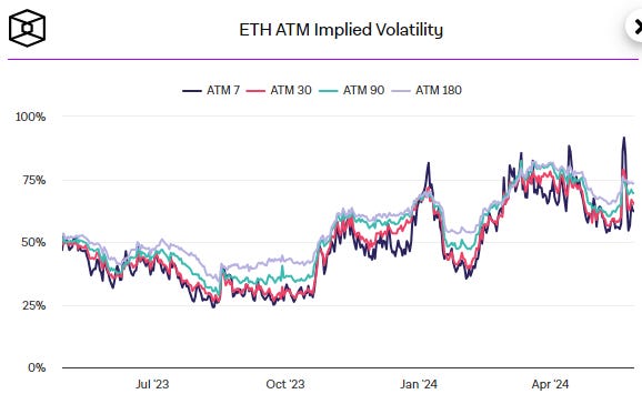
If Panoptic starts calculating pool implied volatilities to highlight attractive pools, this would highlight the LP profitability problem. A 20% fee increase is significant and would flip the profitability sign from negative to positive. As an FYI, I outlined a solution that eliminates this cost entirely. Someday, I'll find someone who thinks eliminating the LP's expense is a good idea.2
If they allocated $10MM in rewards, the PIP:USD ratio is 100:1, meaning 1 PIP is worth 1 cent. Given tokens have decimals, what is the purpose of giving someone 1 cent?
Currently, the people I meet in defi are not sure convexity costs matters, or that it can be eliminated by lower latency, an unknown 'hook,' variable fees, or a different fee level.