Creating a stablecoin position on a perp exchange is hard, but it should be easy. It not only caters to demand, but it also adds liquidity to perp markets that are perpetually short shorts. Here is how to do that.
CEX Stablecoins Good But Risky
The new rapidly growing stablecoin Ethena is built on the fact that natural demand for perp leverage is overwhelmingly on the long side. This generates a fat 11% premium for going short, which can be used to create a riskless return significantly higher than any real world assets like Treasury Bills (5%). Ethena is a sustainable business model in that there is considerable demand for this kind of return, and big crypto exchanges need short open interest and alternatives to the dominant centralized stablecoins Tether and Circle.
Ethena documentation lists a myriad of procedures in their protocol categorized like Russian dolls. Its Internal Services lists five systems, including its Portfolio Management System. Their Hedging System lists a dozen functions, many of which imply considerable discretion, such as determining 'where to route & execute orders upon a successful mint & redeem USDe request.' Access control includes ten entities with smart contract access (gatekeeper, rewarder, EthenaMinting admin, etc.), each of which lists from one to 20 addresses. Each step in their protocol is a centralization point where bad things can happen. With $3B in stablecoins outstanding and only a $33MM(?) insurance fund, a relatively minor mistake would provoke a catastrophic run on the liquidity.
Ethena lists the following risks in their docs: funding, liquidation, custodial, exchange, and collateral. They are all manageable, but we tend to overemphasize what we can measure or at least form a reasonable opinion on, which these are. However, it is the unknown unknowns that are most dangerous. For example, in the 2008 financial crisis, most mortgage derivatives risk assessments focused on diversification and intricately complicated cashflow waterfall mechanisms, taking the aggregate mortgage default rate as a given based on its historically low experience. It had lots of complex correlations by geography, price, etc. that was the focus of financial engineering. Obviously, with the mean default rate constant, it was a well-defined statistical problem.
With hindsight, that was simply a lousy credit risk model, but in real-time, it was an operational risk, as no one thought mortgage default rates would triple their prior historical worst-case scenario. Sure, some people knew strippers were getting mortgages with no money down (as suggested in The Big Short). In contrast, like most people, I had no clue about the deterioration in mortgage underwriting until reading about it after the fact.
Nobelist Robert Shiller created a popular house price index and famously outlined a way to create a perpetual futures for housing prices. In 2008, he claimed to have called the housing crash, but his 2005 edition of Irrational Exuberance merely included the cautiously worded statement that significant further housing price increases "could lead, eventually, to even more significant declines… in some areas." That short, tentative statement—could, in some areas—is contentless. Hindsight bias is ubiquitous and diminishes our appreciation for unknown unknowns.
I hope Ethena emphasizes safety over growth. Unfortunately, many are throwing money at them without qualification (e.g., the Blast L2 is built on MakerDao’s Spark which pledged up to $1B to Ethena), discouraging good habits. So much money is pouring in that slowing things down will cost them millions in income to prevent risks that, in theory, can't happen (their smart contracts are open and audited!). Just as important as their technical knowledge, they need humility and patience, simple but uncommon virtues.
Current DEX Perps are too Risky
OXD and LemmaUSD tried creating a stablecoin on-chain using DEX perps, but these did not work. Part of this was related to scale, as a small stablecoin is not very useful as a medium of exchange, as few people are willing to accept it because it is unfamiliar. The major problem, however, is that DEXes are risky, making them not very comforting when aiming at a risk-free return. The risks of moving assets off-chain are substantial, but at least one can be pretty confident that Binance will not go insolvent. If the collateral can be segregated and the pnl on-exchange is actively swept, there should not be too much CEX counterparty risk.
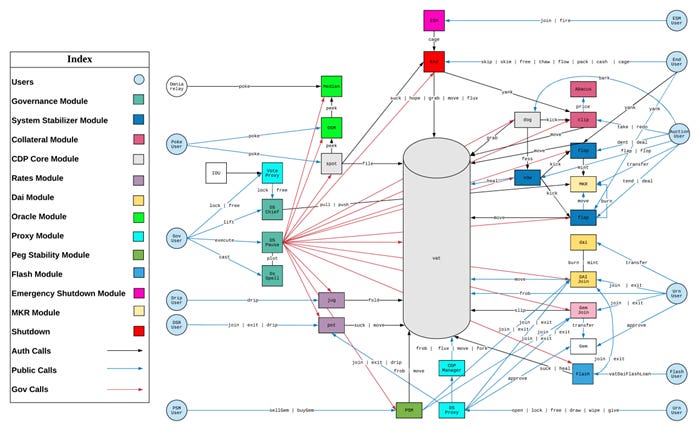
The defi exchanges Euler, Beanstalk, Cream, BonqDAO, BadgerDAO, Sonne Finance, DMM Bitcoin, and Mango Markets all experienced hacks sufficient to ruin any potential stablecoin that might have been built on them. MakerDao is one of the safer protocols in defi, and even its various hacking surfaces defy comprehension. Below is a flow chart they created of who does what and where. I doubt anyone outside of MakerDao fully understands the security for all those rabbit trails.
Perp Dexes have the nasty habit of complicating their protocol. Perp exchange GMX has a liquidity and governance token, both with staked, bonus, and staked&bonus versions. The various rights and responsibilities are difficult to outline and monitor. Pool risk is not siloed into single pools, allowing less liquid tokens that are easier to manipulate to push the entire protocol into insolvency. Incentive programs reminiscent of multi-level marketing scams imply a focus on emulating tradFi UX over security, which does not reassure.
Someday, private blockchain perps like DyDx or Hexalot could be helpful (perhaps when Zksnark people get an epiphany). Currently, however, the risks are significant unless one is intimately familiar with the dapp's personnel. An outside regulator could shut them down, seize the protocol, or make unreasonable demands on users to regain their funds (e.g., prove all your users acquired their funds legally). No amount of auditing can compensate for this centralization risk, where the CEO could mysteriously die doing volunteer work at an orphanage in India, leaving a gaping hole in the protocol's balance sheet. Only an insider would be foolish enough to put more than a million dollars on these exchanges.
Perp-Stable
A robust stablecoin position built on a perp DEX is not only feasible but complementary. Stablecoin positions make perp DEXes better. Long ETH spot and short the perp fit perfectly on a single perp contract with no third parties using a simple AMM. Ideally, a perp DEX should make such positions native to their contracts, eliminating the need for ad hoc tokens, so one can post ETH and short ETH in the same account on a single contract.
Perp-Swap
A perp DEX is also complementary with a standard spot AMM. Swapping ETH for USDC and vice versa is the best way to keep the perp price in line, as arbitrage is finance's most powerful disciplining mechanism. The ability to swap allows liquidators to exit acquired positions quickly at low impact. Many perp DEXes instead rely on oracles and the perp premium to the oracle price as their method of tying their perp price to the spot price. This is a farce and unnecessary, as direct swapping is far more powerful. One can create a funding rate mechanism to equilibrate long and short demand using the relative amounts of long and short user positions, as SNX and GMX do. [This is another reason I do not trust most perp DEXes: their creators are either clueless or being … diplomatic.]
The key to a safe DEX with perp-stablecoin-swap functionality is simplicity. This starts with single pool isolation and not one based on dogwifhat. Targeting the most liquid trading pairs reduces manipulation risk and makes it easier for those with on-contract stablecoin positions to monitor their solvency.
Simple Accounting
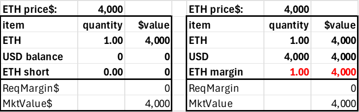
The second simplifying principle is minimizing the number of protocol tokens and account balance fields. The trader's account can consist of three items: the two tokens and the margin position in the risky asset. Only the USD and ETH margin balances can be negative, as shorting ETH implies borrowing ETH, and levering long ETH implies borrowing USD. We separate the ETH into a regular (spot) balance and a margin version to assess relative long-short leverage demand (it’s easier—and simpler—to track using just one side of the margin trades). A trader's account would look as follows.
This is just an AMM where users can have on-contract balances. In standard AMMs only LPs have balances on the contract, the 'total locked value.' Here, the traders have balances on the contract to borrow ETH or USD, which generates a debit to ETH margin or USD.
The market value of the user's account is just USD + net ETH times the price, so this can be calculated when required and needs no state (as the price changes, it would be stale anyway). The required margin is based on the user's net risky position, which is the sum of their ETH collateral and margin, as only the account's net ETH position generates market risk.
Market Value and Required Margin are determined using the price, which, as in AMMs, is a state variable stored in the contract.
netETH = ETH + ETH margin
MarketValue = ETH price * netETH + USD
Required Margin = 0.2 * netETH * ETH price
Here, the maximum leverage is 5, but it could be 2 or 10 (required margin is 1/maxLeverage)
Basics: simple swapping
The contract handles simple swap transactions on contract, so balances are moved from ETH to USD and vice versa. The contract could also handle swaps as AMMs do, allowing users to trade without creating an account. On-contract balances are only necessary for those desiring leverage.
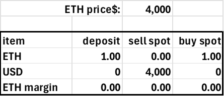
Basics: USD deposit, levers long or short
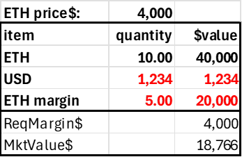
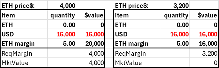
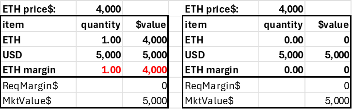
Assume a trader deposits $4000 into his account, where the current ETH price is $4000. With a 20% margin requirement (max leverage 5.0), this trader could go long or short 5 ETH. In practice, this would be reckless, as the account would be subject to liquidation with a high probability, but it shows how the margin requirement corresponds to a price movement. The short 5 ETH position generates $20,000 in USD, and adding this to the initial $4k deposited allows us to calculate the accounts pnl without having an explicit pnl subaccount. Note the account becomes insolvent after a 20% price decline. Ideally, these accounts would be liquidated far before this price movement, but it highlights how the required margin (20%) relates to the 'worst case scenario' in a coin's price risk.
Trader deposits $4,000, shorts 5 ETH
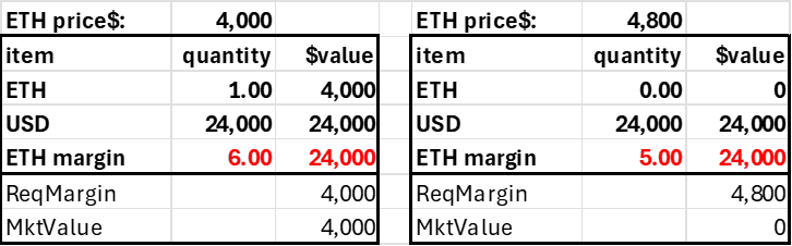
The long 5 ETH position would debit the account's USD field by $20,000. In both cases, the initial trade would not affect the account's total market value (excluding fees and slippage), but with long leverage, the account acquires a negative USD balance. The key is that the account's market value exceeds its required margin or is subject to liquidation.
Trader deposits $4,000, goes long 5 ETH
ETH deposit, levers long or short
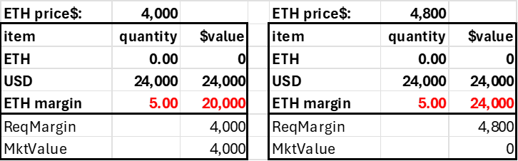
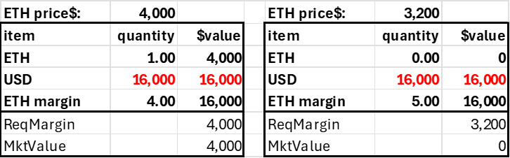
An account created with an ETH deposit is a little trickier because this collateral position either mitigates or accentuates the account's risk. Say the user deposits 1.0 ETH. As the required margin is a function of the account's net ETH position, it has a required margin even though the trader has made no trade. However, this is not a worry as this number will move up and down with the price of ETH and always be 20% of the market value.
With 1.0 ETH in collateral, the trader can short 6 ETH, giving his account a net ETH position of -5. As with the case where $4000 is deposited, the account is solvent up to a 20% price jump.
Trader deposits $4,000 in ETH, goes short 6 ETH
For a long position, the trader can only lever long 4 ETH, giving the account a net ETH position of 5. As in the $4000 deposit case, this account is solvent up to a 20% price decline. In all these cases, we have $4k in value supporting a net $20k position in the risky asset.
Trader deposits $4,000 in ETH, goes long 4 ETH
Closing margin positions
An account with a long 1.0 ETH margin could move that to its regular ETH balance to avoid paying a funding rate or before the withdrawal. Alternatively, it could sell it, and the proceeds would go into USD collateral.
A short ETH margin balance needs either a transfer from the ETH account or buying 1 ETH with USD to eliminate the short position.
Financing Rate
As perp users strongly prefer long over short, the financing rate is necessary to equilibrate demand. We do not need an oracle price to determine a perp premium. Instead, we can use a function based on the DEX's long and short demand. Something like the following, which caps the funding rate at 60%, because if markets are working, that is more than enough:
Long Margin = sum(ETH margin| ETH margin > 0)
Short Margin = - sum(ETH margin| ETH margin < 0)
Total Margin = Long Margin + Short Margin
Rate Paid to Shorts = 0.3 + {LongMargin/(ShortMargin + LongMargin)}* 0.6
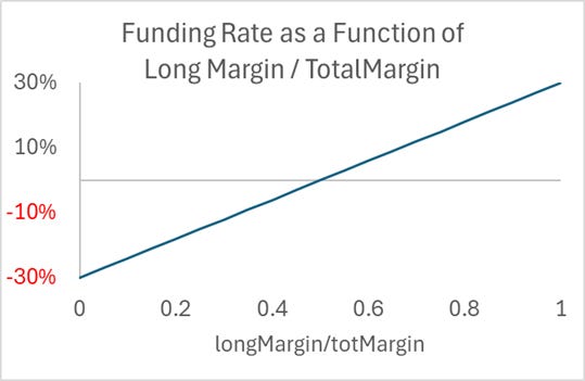
You could put in a sigmoidal curve, but the key is that when long and short demand are equal, the funding rate should be zero.
Insurance Fund/Equity
A standard AMM has zero default risk because no one has leverage. With leverage, users can go insolvent, and if the sum of this insolvency exceeds the contract's insurance fund, the contract has more liabilities than assets. At that point, the first to redeem their assets get paid out in full, while the last gets nothing. This motivates a classic bank run, which leads to panic selling, exacerbating the crisis. A critical part of creating a safe perp DEX consists of
1. A sufficient insurance fund
2. An efficient liquidation process
The insurance fund should be easy to monitor, and the liquidation process should be easy to do.
Initially, the insurance fund must be significant enough to generate user confidence. Realistically, the initial creators would act as both initial liquidity providers and the donors of the initial insurance fund. If the initial insurance fund providers were also liquidity providers, they would have a solid incentive to set up the liquidation bots efficiently to protect themselves. These initial insurance fund providers would get equity tokens, giving them a pro-rata claim to the contract's residual token balance. At first, their equity tokens would be valued at the insurance fund. Investors can reclaim their initial investment without a loss if no one ever shows up.
The insurance fund is the residual capital in the contract, the excess of total assets in the contract over trader and LP assets. Liquidation and fee revenue would accrue to the insurance fund as profits add to a company's retained earnings. The equity tokens could be redeemed for this money, or a user could sell them. As the market value of a prospering contract is greater than its book value, most would choose to sell rather than redeem. At some point, the growth in these residual assets would slow down, and it would be attractive for some to redeem rather than sell these equity tokens. This makes the protocol's end game easy, as when the contract is shut down, the equity token holders would redeem their tokens for the accumulated income and initial capital.
Liquidation
A liquidation mechanism that incents bots to monitor accounts falling below their required margin must exist. Popular CEXes provide over 100-fold leverage, which is infeasible on any decentralized chain and protocol. It's irresponsible to offer this anyway, as crypto is twice as risky as any stock, so amping that up to 200x riskier is just a way of harvesting liquidation revenue from inexperienced traders. As the ETH price moved 10% on May 20, 2024, in only 15 minutes, and moved by 20% on March 12, 2020, a leverage limit of 5 on ETH or BTC should minimize the number of insolvencies to trivial levels that the insurance fund should cover.
A liquidator should always receive an insolvency fee, as without the profit motive, we cannot depend on them, and insolvent accounts are precisely the sorts of accounts we want to prioritize. Ideally, the same liquidator fee should go to the DEX to help build its insurance fund. Consider the following account that is below its required margin.
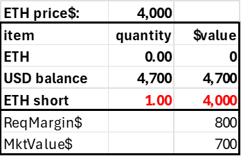
Assume the liquidation fee is 10% of the risky position liquidated, here 1 ETH worth $4000. The defaulter pays a fee split 50:50 between the insurance fund and the liquidator. It would be something like 10%, applied to the notional amount at risk.
liqFee= 0.1 * abs(ETH Margin)*ETHprice
The liquidator acquires the defaulter's ETH margin position, offset by an offsetting debit or credit to his USD account, a net value of zero. The liquidation fee in USD is added to the liquidator's USD balance.
cash flow for liquidator

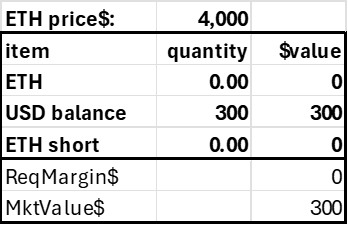
The defaulter’s account gets his risky ETH margin position zeroed out, and either the residual USD value of this position minus the liquidation fee is added to his USD position, or zeroed out if the defaulter’s account value is negative.
Balance Sheet for Defaulted Account

The insurance fund, or contract equity, receives either the liquidity fee or is debited to absorb the cost of an insolvent account (the negative value of the account after paying the liquidator).
Cash Flow to Contract

So, for the above account, the ETH and USD balances would change as follows:
This generates the following result on the defaulter's account.
For an insolvent account, like this:

The resulting coin flows would be as follows:
This corresponds to the liquidator receiving his 200 USD reward for liquidation, zeroing out the defaulting account (debiting his entire $3000, and debiting the insurance fund to account for the insolvency and the fee paid to the liquidator).
As long as the liquidation bots are working, all accounts with insufficient margin should have been liquidated. If so, tracking account balances this way makes it easy for an outsider to see if the contract is solvent, as the insurance fund's USD and ETH accounts keep a score of the accumulated insolvency debits and credits and trade fees relative to the initial insurance fund balances. The insurance fund balance is a singular state variable available in a getter function.
By having the liquidator acquire the defaulter's position instead of automatically trading it on the DEX, the liquidator has the discretion to avoid losing money exiting the position at a bad price. Specifically, if the position size is significant, the liquidator should prefer to parcel out the acquired position piecemeal to avoid a significant market impact (arbs would push the price back up after each sale with a major price impact).
Note the liquidator would be insufficiently margined when acquiring this position if they had zero money in their account, as the liquidation fee is 5% while the required margin is 20%. A liquidation bot will need an account with adequate capitalization to handle significant insolvencies, and allowing liquidators to take portions of the defaulter's position could help here. One can add other nuances, such as using a moving average price when triggering liquidation, but the point here is that liquidation is straightforward and amenable to automation.
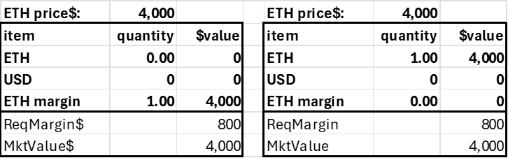
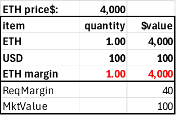
Stablecoin position
The stablecoin position is an account funded by ETH that shorts the same amount of ETH. Note the required margin is zero, as the position has no risk from ETH price changes.
Post 1 ETH Create Stablecoin Position
The $4000 generated by the short position implies this account could afford to withdraw all its USD, generating positive funding with zero capital. As funding rates can go negative, that's not a good idea, so it's necessary to have an auxiliary minimum capital amount based on the absolute value of the ETH positions, but that's a straightforward adjustment. Even if the funding rate was 52%, that's only a predictable 1% change in the account's value over a week compared to a 3% daily ETH price variability, and we can see how the stablecoin position is not risky.
So, in practice, a required margin would be something like the following:
Required Margin = max[0.01*abs (ETH margin)*ETH price,
0.2*abs(netETH) * ETH price]
Post 1 ETH, withdraw 97.5% of its value in USD
Get funding rate on short 1 ETH Risk-Free
Here, the prudent stablecoin account holder has 2.5 times the required margin and gets the full short funding with only 2.5% capital applied. He could then do this again and again, That is,
deposit 1.0 ETH, short 1.0 ETH, withdraw 3900 USD, buy 0.975 ETH
deposit 0.975 ETH, short 0.975 ETH, withdraw 3802.5 USD, buy 0.9506 ETH
deposit 0.95063 ETH, etc.
With no transaction costs, you can create 40 ETH worth of stablecoin positions for only 1 ETH. With transaction costs, say it’s 20 times. That implies the standard 11% short funding rate would generate a 220% return, risk free.
With a 30% funding rate cap, the account holder can safely ignore his account for weeks and be assured his stable position cannot be liquidated. In contrast, with USD collateral for a short position, the stablecoin position requires cash flow into and out of the perp account to counter the day's ETH price movement, which averages 3%. Extra transactions increase risk, as on the blockchain, one cannot reverse charges as they do in tradFi, so each admin transfer managing the daily pnl, common on many perp exchanges, is a potential disaster.
This capital efficiency would probably drive funding rates down to something reasonable, as 10% is not an equilibrium, let alone the 20%+ funding rates we often see. A ceiling for an equilibrium rate for such a low-risk position would be the equity premium, which is around 3-5% above the risk-free rate.
Why Not?
I am not sure why Uniswap or one of their alternatives is not doing this, as it would give users access to the standard AMM and so much more. I wrote about this two years ago, but clearly, just as much as AMMs don’t care about—let alone want to remove—the LP’s IL/LVR, DEXes don’t care about solving two problems at once (short OI and easy stablecoin position). I would love to see a perp DEX where I could short or use to harvest the short funding rate risk-free, but I don't trust any of them.
I suspect a primary reason many big AMMS haven’t added this feature is regulation. Simply swapping tokens is somewhat of a gray area for regulators, as it is not clear whether tokens are securities, commodities, or something else. Anything offering leverage is more clearly covered by derivatives regulation, such as the CFTC's Swap Execution Facility. If Uniswap built a perp dex, regulators would be given the attack surface they have been looking for. An official protocol giving leverage would have to be domiciled in the Seychelles, Israel, or Mongolia. A stable-perp-swap DEX could be run as a genuinely autonomous contract so that there is no one but a variable set of pseudonymous users to prosecute. While this is feasible, it would not appeal to VCs, who tend to be incorporated in countries with active regulators.
[I did not address how the LPs fit into this, but this post is long enough. I also just explained the stablecoin position instead of its potential use as a medium of exchange in this framework. Perhaps later.]
