About half of Robeco’s Quantitative Investing team recently published a short paper on monthly trading strategies (see Blitz et everybody Beyond Fama-French Factors: Alpha from Short-Term Signals Frequencies). I can imagine these guys talking about this stuff all the time, and someone finally says, “this would make a good paper!”
‘Short-Term’ refer to one-month trading horizons. Anything shorter than a month does not significantly overlap with standard quant factors like ‘value’ because they involve different databases: minute or even tick data, level 2 quotes. They are less scalable and involve more trading, making them more the province of hedge funds than large institutional funds. Alternatively, super-short-term patterns can be subsumed within the tactics of an execution desk, where any alpha would be reflected in lower transaction costs.
The paper analyzes the five well-known anomalies using the MSCI World database, which covers the top 2000 largest traded stocks in developed countries.
Monthly mean-reversion. See Lehman (1988). A return in month t implies a low return in month t+1.
Industry momentum. See Moskowitz and Grinblatt (1999). This motivates the authors to industry-adjust the returns in the mean-reversion anomaly mentioned above so it becomes more independent.
Analyst earnings revisions over the past month. See based Van der Hart, Slagter, and van Dijk (2003). This signal uses the number of upward earnings revisions minus the number of downward earnings revisions divided by the total number of analysts over the past month. It is like industry momentum in that it implies investor underreaction.
Seasonal same-month stock return. See Heston and Sadka (2008). This strategy is based on the idea that some stocks do well in specific months, like April.
High one-month idiosyncratic volatility predicts low returns. See Ang, Hodrick, Xing, and Zhang (2006). This will generally be a long low-vol, short high-vol portfolio.
All of these anomalies initially documented gross excess monthly returns of around 1.5%, which, as expected, are now thought to be a third of that at best; at least they are not zero, as is the fate for most published anomalies.
Interestingly, Lehmann’s paper documented the negative weekly and monthly autocorrelation that underlay the profitable ‘pairs-trading’ strategy that flourished in the 1990s. Lo and Mackinlay also noted this pattern in 1988, though their focus was testing random walks, so you had to read between the lines to see the implication. DE Shaw made a lot of money trading this strategy back then, so perhaps Bezos funded Amazon with that strategy. A popular version of this was pairs trading, where for example, one would buy Coke and sell Pepsi if Coke went down while Pepsi was flat. Pairs trading became much less profitable around 2003, right after the internet bubble burst. However, this is a great example of an academic paper that proved valuable for those discerning enough to see its real value (note that Lehmann’s straightforward strategy was never a highly popular academic paper).
An aside on DE Shaw. While making tons of money off of this simple strategy, they did not tell anyone about it. They would tell interviewees they used neural nets, a concept like AI or machine-learning today: trendy and vague. I have witnessed this camouflage tactic firsthand several times, where a trader’s edge was x, but he would tell others something plausible unrelated to x. Invariably, the purported edge was more complicated and sophisticated than the real edge (e.g., “I use a Kalman filter to estimate latent high-frequency factors that generate dynamic alphas” vs. “I buy 50 losers and sell 50 winners every Monday using last week’s industry-adjusted returns”).
If each strategy generates a 0.5% monthly return, it is interesting to think about how well all of them do when combined. Below is a matrix of the correlation of the returns for these single strategies. You can see that by using an industry-adjusted return, the monthly mean-reversion signal becomes significantly negatively correlated with industry momentum. While I like the idea of reducing the direct offsetting effects (high industry returns —> go long; high returns —> go short), I am uncomfortable with how high the negative correlation is. In finance, large correlations among explanatory variables suggest redundancy and not efficient diversification.
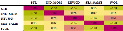
STR=short-term mean reversion, IND_MOM=industry momentum, REV30D=analyst revision momentum, SEA_SAME=seasonal same month, iVOL=one-month idiosyncratic volatility.
Their multifactor approach normalizes their inputs into Winsorized z-scores and adds them up. This ‘normalize and add’ approach is a robust way to create a multifactor model when you do not have a strong theory (e.g., Fama-French factors vs Black-Scholes). Robyn Dawes made a case for this technique here. His paper was included in Kahneman, Slovic, and Tversky’s seminal Judgment under Uncertainty, a collection of essays on bias published in 1982. In contrast, multivariate regression weights (coefficients) will be influenced by the covariances among the factors as well as the correlation with the explanatory variable. These anomalies are known only for their correlation with future returns, not their correlations with each other. Thus, excluding their correlation effects ex ante is an efficient way of avoiding overfitting, in the same way that a linear regression restricts but dominates most other techniques (simple is smart). The key is to normalize the significant predictors into comparable units (e.g., z-scores, percentiles) and add them up.
I should note that famed factor quant Bob Haugen applied the more sophisticated regression approach to weighting factors in the early 2000s, and it was a mess. This is why I do not consider Haugen the OG of low vol investing. He was one of the first to note that low volatility was correlated with higher-than-average returns, but he buried that finding among a dozen other factors, each with several flavors. He sold my old firm Deephaven a set of 50 factors circa 2003 using rolling regressions, and the factor loading on low vol bounced from positive to negative; the model promoted historical returns of 20+% every year for the past 20 years, while never working while I saw it.
I am not categorically against weighting factors; I just think a simple ‘normalize and add’ approach is best for something like what Robeco does here, and in general one needs to be very thoughtful about restricting interaction effects (e.g., don’t just throw them into a machine learning algorithm).
The paper documents the transaction costs that would make the strategy generate a zero return to handle this problem. This has the nice property of adjusting for the fact that some implementations have a lower turnover than others, so that aspect of the strategy is then included within the tests. The y-axis in the chart below represents the one-way transaction costs that would make the strategy generate a zero excess return. Combining signals almost doubles the returns, which makes sense. You should not expect an n-factor model to be n times better than a 1-factor model.
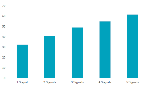
They note some straightforward exit rules that reduce turnover, and thus transaction costs, more than it lowers the top-line returns. Thus, in the chart below, no single anomaly can overcome its transaction costs, but a multifactor approach can. Further, you can make straightforward adjustments to entry and exit rules that increase the net return even while decreasing the gross return (far right vs. middle columns).
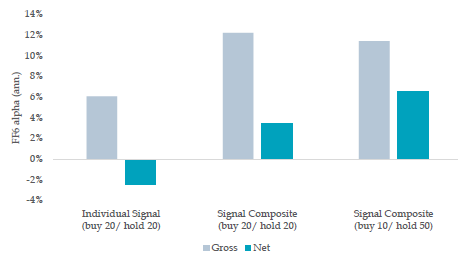
They also present data on the long-only implementation and find the gross excess return to fall by half, suggesting the results were not driven by the short side. This is important because it is difficult to get a complete historical dataset of short borrow costs, and many objectively bad stocks cannot be shorted at any rate.
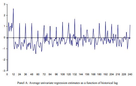
I am cautious about their results for a couple of reasons. First, consider the chart below from the Hesten and Sadka (2006) paper on the monthly seasonal effect. This shows the average lagged regression weighting on prior monthly returns for a single stock. Note the pronounced 12-month spike, as if a stock has a particular best month that persists for 20 years. The stability of this effect over time looks too persistent to be true, suggesting a measurement issue more than a real return.
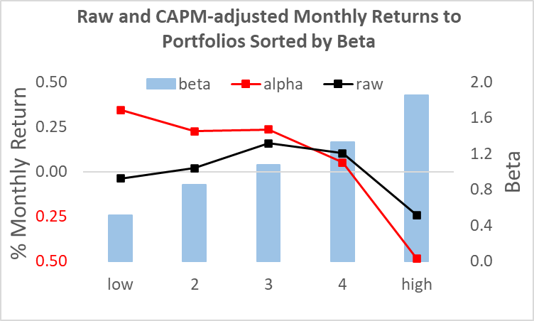
Another problem in this literature is that presenting the ‘alphas’ or residuals to a factor portfolio is often better thought of as a reflection of a misspecified model as opposed to an excess return. Note that the largest factor in these models is the CAPM beta. We know that beta is at best uncorrelated with cross-sectional returns. Thus, you can easily generate a large ‘excess return’ merely by defining this term relative to a prediction everyone knows has a systematic bias (i.e., high beta stocks should do better, but don’t). You could create a zero-beta portfolio, add it to a beta=1.0 portfolio and seemingly create a dominant portfolio, but that is not obvious. The time-varying idiosyncratic risk to these tilts does not diversify away and could reduce the Sharpe of a simple market portfolio.
Interestingly, Larry Swedroe recently discussed a paper by Medhat and Schmeling (2021). They found that monthly mean reversion only applies to low turnover stocks; for high turnover stocks, the effect is to find its opposite month-to-month momentum. I do not see that, but this highlights the many degrees of freedom in these studies. How do you define ‘excess’ returns? What is the size cut-off in your universe? What time period did you use? Did you include Japan (their stock market patterns are as weird as their TV game shows)?
Robeco’s paper provides a nice benchmark and outlines a straightforward composite strategy. If you are skeptical, you might simply add them to your entry and exit rules.
1 comment:
"In contrast, multivariate regression weights (coefficients) will be influenced by the covariances among the factors as well as the correlation with the explanatory variable."
You don't need regression, per se. It obviously depends on assumptions you are making, but in the simplest case you just need expected returns of each factor. From this, you can produce expected returns of each stock. if you assume that the expected returns of each factor are equal, then the resulting expected returns of each stock are just a linear transformation of the sum of the individual factor scores.
Anyway, if regressions are a mess, use regularization or Bayesian techniques to impose a prior.
Post a Comment